DiskANN 系统
1. 为什么需要 DiskANN
前面的 HNSW 和 Vamana 章节关注的是“怎样沿图找到候选”,没有讨论这些数据具体放在哪里。当数据规模继续增大时,图和原始向量可能无法全部放进内存,只能把体积较大的部分放到 SSD(固态硬盘)中。
SSD 的容量通常比内存大,但随机读取更慢。如果每展开一个节点都要单独等待一次 SSD 读取,查询延迟就会被一轮轮等待拉长。DiskANN 的做法说白了就是三招:能放内存的尽量放内存,内存快;必须放硬盘的,攒成一批一起读,别让硬盘来回跑;读回来之前,先用压缩过的小数据把候选粗排一遍。分工上,Vamana 的图负责带路,PQ 的压缩向量负责粗排,SSD 存完整数据。
2. 数据存储分工
2.1 内存里的数据
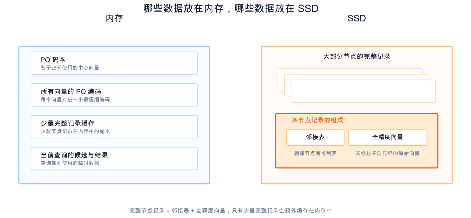
内存里放这三样:
- PQ 码本和每个向量的 PQ 压缩表示;
- 少量节点记录的内存副本(缓存);
- 当前查询的候选和结果。
内存中的 PQ 压缩表示体积较小,用来估算已经发现的候选离查询向量有多近。PQ 不会先扫描全库,也不负责最终结果;编码和距离计算可参考 PQ 算法教程。
缓存的规矩很简单:内存里留了副本的点,直接用内存里的,不碰 SSD;没留副本的点,才去 SSD 读。留给谁?一般是离入口几步路以内的那批点(论文取 3 到 4 跳),因为搜索刚开始的那几步几乎每条查询都要走;也可以干脆统计谁被读得最多就留谁。这个范围不能放宽太多:多放宽一跳,要留的节点就涨得飞快。
2.2 SSD 节点记录
SSD 上存的是每个节点的“完整档案”。读 SSD 有个特点:一次最少读一页,哪怕你只要一个字节,也得等一整页的时间。所以 DiskANN 干脆把每个节点的两样东西——邻居名单和完整向量——钉在同一页档案里:翻一次档案,既知道下一步往哪走(邻居名单),又顺手把这个点的真实距离记下来(完整向量)。每个节点最多 R 个邻居,每份档案多厚也就定死了。查询结束时,最终结果就在这些已经读过的真实距离里挑前 k 个,不用再碰 SSD。
3. 索引怎样建出来
3.1 建图流程
本章只讨论一次性构建的索引,不涉及在线更新。
构建做四件事:
- 训练 PQ。 用数据集算出码本,再给每个向量写下压缩编码。
- 用 Vamana 建图。 沿用上一章的单层图,每个节点最多
R条出边。 - 把节点写成 SSD 记录。 每个节点一条,格式见 2.2。
- 复制一批节点到缓存。 缓存范围见 2.1。
3.2 建图内存限制
先把两件事分开:第 2 节说的是“查询的时候数据放不进内存”,这一节说的是“建图的时候内存就不够用”。本章示例的数据不大,图在内存里就能建完。真到了内存装不下的时候,论文的做法是把数据切成几片、每片各建一张图、最后把图拼到一起;本章不实现这一步,知道有这回事就行。
4. 查询流程
4.1 基本概念
- 候选:搜索已经发现、可能接近查询向量的节点;
- 展开:读取一个候选的完整记录,并沿它的邻接表发现更多节点;
- top-k:最终返回的结果个数。
W 是一轮最多选多少个候选。L 是候选列表最多留多少个节点。
4.2 候选展开循环
查询从图的入口节点开始,并重复下面的过程:
- 用 PQ 近似距离排列当前已经发现的候选;
- 按这个顺序跳过已经展开的候选,最多选择
W个; - 命中缓存的记录直接从内存取得,其余记录在同一轮从 SSD 读取;
- 用邻接表发现新候选,并记下全精度距离;
- 合并旧候选和新候选,按 PQ 近似距离只保留前
L个; - 保留列表里还有未展开的节点,就回到第 1 步;否则从已经展开的节点中按全精度距离取前
k个。
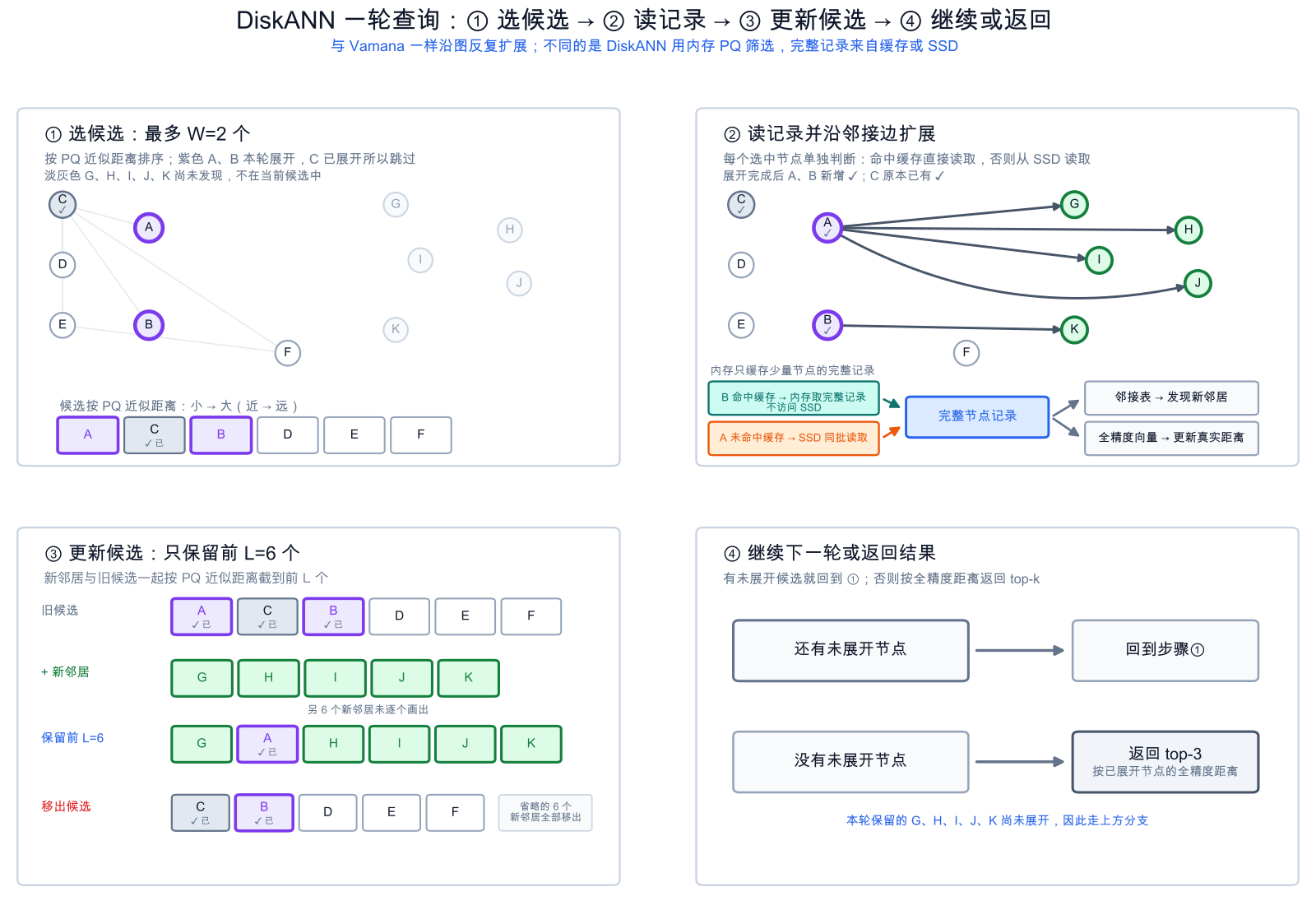
看图时记住一点:同一个字母永远是同一个节点。③对应第 5 步——按 PQ 距离只留前 L 个,这决定的是“谁能留在候选名单里”,还不是最终排名。最终结果只看已经展开过的点(C、B)的真实距离;没挤进名单的 D、E、F 这轮就出局了,不会再被展开;A 虽然还留在名单里,但它已经展开过,不会再展开第二次。
4.3 结果与近似性
真实距离只在展开过的点上算过;没被展开的点只是“没轮到”,并不能证明它们更远。所以最终结果可能错过真正的最近邻,DiskANN 仍然是近似搜索。
5. 教学实现
配套 Notebook:src/ANN_alorithms/DiskANN系统.ipynb。
下面的实现复用上一章的 SimpleVamana 建图。
配套 notebook 在 src/ANN_alorithms 目录下运行,才能 from vamana import SimpleVamana。
5.1 数据与 Vamana 图
示例只缓存入口和邻接表里的前三个邻居。
import numpy as np

from vamana import SimpleVamana


def make_dataset(seed=7, n_per_cluster=10, dimension=8):
    rng = np.random.default_rng(seed)
    coords = np.linspace(-27.5, 27.5, 12)
    centers = np.stack([coords, np.zeros(12)], axis=1)
    rows = []
    for center in centers:
        xy = rng.normal(loc=center, scale=0.8, size=(n_per_cluster, 2))
        derived = np.column_stack([
            xy[:, 0] * 0.35 + xy[:, 1] * 0.20,
            xy[:, 0] * -0.15 + xy[:, 1] * 0.40,
        ])
        noise = rng.normal(scale=0.15, size=(n_per_cluster, dimension - 4))
        rows.append(np.column_stack([xy, derived, noise]))
    return np.vstack(rows).astype(np.float32)


X = make_dataset()
vamana = SimpleVamana(R=10, L_build=24, alpha=1.1, seed=7).fit(X)
graph, entry = vamana.graph, vamana.entry
cache_nodes = {entry, *graph[entry][:3]}5.2 查询模拟器
DiskANNQuerySimulator.fit 训练 PQ,用字典保存每条 SSD 记录,并把缓存节点的记录留在内存。search 按第 4 节执行。SSD 读取数是一共读了多少条记录。读取轮数只统计发生过 SSD 读取的轮,全部命中缓存的轮不计。SSD 记录放在字典里,我们通过如下的方式进行耗时模拟的对比:读了 SSD 的每一轮先算 100,这一轮读出几条记录,每条再加 10,即 io_rounds × 100 + ssd_reads × 10。
class DiskANNQuerySimulator:
    """模拟 DiskANN 查询:内存中用 PQ 排列候选,按需读取 SSD 上的节点记录。"""

    def __init__(self, graph, entry, pq_subspaces=4, pq_centroids=8,
                 kmeans_iters=15, cache_nodes=()):
        self.graph = graph
        self.entry = entry
        self.pq_subspaces = pq_subspaces
        self.pq_centroids = pq_centroids
        self.kmeans_iters = kmeans_iters
        self.cache_nodes = set(cache_nodes)

    def _kmeans(self, data):
        init = np.linspace(0, len(data) - 1, self.pq_centroids, dtype=int)
        centers = data[init].copy()
        for _ in range(self.kmeans_iters):
            distances = ((data[:, None, :] - centers[None, :, :]) ** 2).sum(axis=2)
            labels = np.argmin(distances, axis=1)
            for c in range(self.pq_centroids):
                members = data[labels == c]
                if len(members):
                    centers[c] = members.mean(axis=0)
        return centers

    def fit(self, X):
        X = np.asarray(X, dtype=np.float32)
        if X.shape[1] % self.pq_subspaces != 0:
            raise ValueError("向量维度必须能被 pq_subspaces 整除")
        self.sub_dim = X.shape[1] // self.pq_subspaces

        # 内存:每个子空间一个 PQ 码本,每个向量一行 PQ 编码。
        self.codebooks, codes = [], []
        for part in range(self.pq_subspaces):
            sub = X[:, part * self.sub_dim:(part + 1) * self.sub_dim]
            codebook = self._kmeans(sub)
            self.codebooks.append(codebook)
            distances = ((sub[:, None, :] - codebook[None, :, :]) ** 2).sum(axis=2)
            codes.append(np.argmin(distances, axis=1))
        self.pq_codes = np.column_stack(codes).astype(np.uint8)

        # SSD:每个节点一条记录,同时保存全精度向量和邻接表。
        self.ssd_records = {
            node: {"vector": X[node], "neighbors": list(neighbors)}
            for node, neighbors in enumerate(self.graph)
        }
        # 缓存:少量节点记录在内存中的副本。
        self.record_cache = {node: self.ssd_records[node] for node in self.cache_nodes}
        return self

    def _pq_distances(self, table, nodes):
        codes = self.pq_codes[np.asarray(nodes, dtype=int)]
        return table[np.arange(self.pq_subspaces), codes].sum(axis=1)

    def search(self, query, k=5, W=4, L=24):
        query = np.asarray(query, dtype=np.float32)
        # PQ 距离表:查询向量每一段到对应码本中各质心的距离。
        table = np.stack([
            ((query[p * self.sub_dim:(p + 1) * self.sub_dim] - self.codebooks[p]) ** 2).sum(axis=1)
            for p in range(self.pq_subspaces)
        ])
        candidates = {self.entry: self._pq_distances(table, [self.entry])[0]}
        seen = {self.entry}
        expanded, exact = set(), {}
        stats = {"ssd_reads": 0, "io_rounds": 0, "cache_hits": 0, "rounds": []}

        while True:
            # 按 PQ 近似距离排列,跳过已展开的候选,最多选 W 个。
            selected = sorted(
                (node for node in candidates if node not in expanded),
                key=lambda node: (candidates[node], node),
            )[:W]
            if not selected:
                break
            cached = [node for node in selected if node in self.record_cache]
            from_ssd = [node for node in selected if node not in self.record_cache]
            stats["cache_hits"] += len(cached)
            stats["ssd_reads"] += len(from_ssd)
            stats["io_rounds"] += int(bool(from_ssd))

            new = []
            for node in selected:
                if node in self.record_cache:
                    record = self.record_cache[node]
                else:
                    record = self.ssd_records[node]
                expanded.add(node)
                # 用全精度向量计算距离;邻接表带来新候选。
                exact[node] = float(np.linalg.norm(query - record["vector"]))
                neighbors = record["neighbors"]
                for neighbor, distance in zip(neighbors, self._pq_distances(table, neighbors)):
                    if neighbor not in seen:
                        seen.add(neighbor)
                        new.append(neighbor)
                    candidates[neighbor] = distance

            # 新旧候选合并后,按 PQ 近似距离只保留前 L 个。
            kept = sorted(candidates, key=lambda node: (candidates[node], node))[:L]
            candidates = {node: candidates[node] for node in kept}
            stats["rounds"].append({
                "selected": selected, "cached": cached, "ssd": from_ssd,
                "new": new, "kept": kept,
            })

        # 在展开过的节点中按全精度距离取前 k 个。
        stats["expanded_nodes"] = len(expanded)
return sorted(exact, key=lambda node: (exact[node], node))[:k], stats5.3 查看一次查询的轨迹
这一节看一条查询的第 2 轮:选中了哪些候选,哪些在缓存里,哪些要读 SSD。W 是一轮最多选多少个候选,L 是候选列表最多留下多少个节点。这一轮仍是 W=2、L=6。
index = DiskANNQuerySimulator(graph, entry, cache_nodes=cache_nodes).fit(X)

query_rng = np.random.default_rng(7)
query_ids = [90, 0, 110, 20]
noise = query_rng.normal(scale=0.08, size=(len(query_ids), X.shape[1]))
queries = X[query_ids] + noise.astype(np.float32)

print(f"dataset: {X.shape[0]} vectors x {X.shape[1]} dimensions")
print(f"entry: {entry}; cached nodes: {len(cache_nodes)}")运行结果:
dataset: 120 vectors x 8 dimensions
entry: 50; cached nodes: 4result, stats = index.search(queries[0], k=3, W=2, L=6)
round_2 = stats["rounds"][1]
print("top-3:", result)
print("round 2 selected:", round_2["selected"])
print("cache hits:", round_2["cached"])
print("SSD reads:", round_2["ssd"])
print("new candidates:", round_2["new"])
print("kept after prune:", round_2["kept"])运行结果:
top-3: [90, 98, 91]
round 2 selected: [62, 64]
cache hits: [62]
SSD reads: [64]
new candidates: [66, 63, 60, 69, 61, 79, 72]
kept after prune: [63, 72, 79, 66, 62, 60]第 2 轮选中 62 和 64,62 命中缓存,64 从 SSD 读取。kept 按 PQ 距离只保留 L=6 个候选,64 在这次裁剪中被移出。64 展开时已记录到查询的全精度距离。查询结束后只从有这项记录的节点中选取 top-3,得到 [90, 98, 91]。
5.4 调整每轮选取上限
先固定 L=6,把 W 依次设为 1、2、4。对 4 条查询取平均,查看每轮选取上限变化后,recall@5、SSD 读取条数、读取轮数和模拟耗时的变化。
def recall_at_k(X, query, result, k):
    truth = np.argsort(np.linalg.norm(X - query, axis=1), kind="stable")[:k]
    return len(set(result) & set(truth)) / k


print(f"查询数:{len(queries)}")
print("L:6")
print(" W  recall@5  SSD读取条数  读取轮数  模拟耗时")

for W in (1, 2, 4):
    recalls = []
    reads = []
    rounds = []
    for query in queries:
        result, stats = index.search(query, k=5, W=W, L=6)
        recalls.append(recall_at_k(X, query, result, k=5))
        reads.append(stats["ssd_reads"])
        rounds.append(stats["io_rounds"])

    avg_recall = np.mean(recalls)
    ssd_reads = np.mean(reads)
    io_rounds = np.mean(rounds)
    sim = io_rounds * 100 + ssd_reads * 10
print(f"{W:2d} {avg_recall:.3f} {ssd_reads:5.2f} {io_rounds:5.2f} {sim:7.1f}")运行结果:
查询数:4
L:6
 W  recall@5  SSD读取条数  读取轮数  模拟耗时
 1  0.600      10.00        10.00    1100.0
 2  0.750      11.75         6.50     767.5
4 0.750 19.00 6.75 865.0| W | recall@5 | SSD读取条数 | 读取轮数 | 模拟耗时 |
|---|---|---|---|---|
| 1 | 0.600 | 10.00 | 10.00 | 1100.0 |
| 2 | 0.750 | 11.75 | 6.50 | 767.5 |
| 4 | 0.750 | 19.00 | 6.75 | 865.0 |
W=2 和 W=4 的召回都是 0.750,W=1 是 0.600。三档里模拟耗时最低的是 W=2,为 767.5;W=4 升到 865.0。
5.5 调整列表保留上限
候选列表允许留下更多节点时,召回能提高多少,SSD 读取条数、读取轮数和模拟耗时又会怎样变化?这里固定 W=2,让 L 依次取 4、8、12、24,查看这 4 条查询的平均 recall@5、SSD 读取条数、读取轮数和模拟耗时。
print(f"查询数:{len(queries)}")
print("W:2")
print(" L  recall@5  SSD读取条数  读取轮数  模拟耗时")

for L in (4, 8, 12, 24):
    recalls = []
    reads = []
    rounds = []
    for query in queries:
        result, stats = index.search(query, k=5, W=2, L=L)
        recalls.append(recall_at_k(X, query, result, k=5))
        reads.append(stats["ssd_reads"])
        rounds.append(stats["io_rounds"])

    avg_recall = np.mean(recalls)
    ssd_reads = np.mean(reads)
    io_rounds = np.mean(rounds)
    sim = io_rounds * 100 + ssd_reads * 10
print(f"{L:2d} {avg_recall:.3f} {ssd_reads:5.2f} {io_rounds:5.2f} {sim:7.1f}")运行结果:
查询数:4
W:2
 L  recall@5  SSD读取条数  读取轮数  模拟耗时
 4  0.600      10.50         6.25     730.0
 8  0.800      13.25         7.25     857.5
12  0.850      16.25         8.75    1037.5
24 1.000 27.25 14.00 1672.5| L | recall@5 | SSD读取条数 | 读取轮数 | 模拟耗时 |
|---|---|---|---|---|
| 4 | 0.600 | 10.50 | 6.25 | 730.0 |
| 8 | 0.800 | 13.25 | 7.25 | 857.5 |
| 12 | 0.850 | 16.25 | 8.75 | 1037.5 |
| 24 | 1.000 | 27.25 | 14.00 | 1672.5 |
增大 L 后,召回从 0.600 提高到 1.000,SSD 读取条数和读取轮数增加。模拟耗时从 730.0 增到 1672.5。