Chapter 2 Introduction to Inference

Next-generation AI development tools, such as Claude Code and Codex, can connect to different LLM APIs, yet the actual user experience still varies considerably. More capable models usually deliver higher task-completion rates, more stable reasoning, and better code quality. Response speed, throughput, and cost also have a direct impact on development efficiency.

Understanding the LLM inference process helps explain how models generate outputs and makes it possible to analyze the key factors that affect inference quality, speed, throughput, and cost. This provides a foundation for inference optimization.

1 Learning Objectives

The previous chapter introduced the overall architecture of LLMs. Inference is the core stage that determines their usability, cost, and development experience. This chapter starts from the principles of inference, breaks down the process layer by layer, and connects it to real-world scenarios. We will investigate the following questions:

• What are the fundamental differences and connections between training and inference in terms of objectives, computation patterns, and resource requirements?
• What is the complete life cycle of a token?
• What responsibilities do the prefill and decode stages have, and why do their characteristics differ so sharply?
• Which factors affect the observed performance of LLM inference?
• How can we determine whether an inference workload is compute-bound or memory-bound?
• Where do bottlenecks arise in scenarios such as Agent collaboration and multi-turn conversations?

After completing this chapter, you should understand the two key stages of inference, use the Roofline model to analyze performance bottlenecks, and select appropriate optimization strategies for specific scenarios.

2 What Is Inference?

We use LLMs to chat, write code, or perform tasks after deploying them in real-world applications. The process by which a model generates an output from a user input is called inference.

A complete LLM inference process can be summarized as follows: the user input first passes through a tokenizer and is converted into token IDs, then enters the transformer through an embedding layer. Using mechanisms such as self-attention, the model computes a representation of the current context and predicts the next token. The newly generated token is fed back as part of the next input, and the process repeats. This is an autoregressive process that continues until the output is complete or a stopping condition is triggered.

This process can be compared to baking a cake: the user's request is the "ingredients," LLM inference is the "processing," and the final sequence of output tokens is the "cake." However, the LLM does not process the entire result in one step; it generates the result one token at a time.

An LLM's capabilities are not created during inference. They are acquired mainly during training through computation over large amounts of data. Inference simply performs forward computation with a trained model. To understand this, we need to clarify the relationship between training and inference and how they differ.

3 Inference and Training

In an LLM's life cycle, training and inference are separate stages with fundamentally different computation patterns: training optimizes parameters in parallel, while inference produces outputs sequentially. Training determines the model's capability boundary; inference exposes problems in real scenarios (alignment deviations, efficiency bottlenecks, and so on). These observations drive targeted improvements on the training side through methods such as RLHF, synthetic data, and distillation.

Together they form a loop: training shapes capabilities, inference makes those capabilities useful, and inference can also guide the evolution of training.

3.1 Differences Between Inference and Training

Both training and inference involve the model's forward computation, but their objectives, computation patterns, and resource bottlenecks are fundamentally different. For either autoregressive inference or parallelized training, suppose the model needs to generate the $i$-th token. The conditional probability at that position can be written uniformly as:

$$P({\text{token}}_i\mid {\text{token}}_1,{\text{token}}_2,\dots ,{\text{token}}_{i-1})$$

The mathematical form of a single-step prediction is the same in training and inference: both estimate a probability distribution over the vocabulary. The difference lies in the source of the preceding context (ground-truth labels versus model-generated tokens) and whether outputs can be parallelized.

Comparison of the inputs used to predict the next token during training and inference

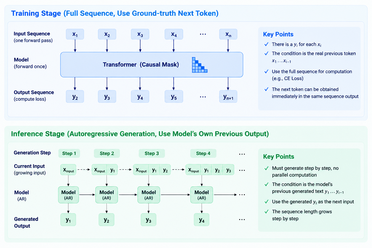
Figure 1. Training vs. inference

Stage	Input source for predicting $toke{n}_i$
Training	The ground-truth sequence from labeled data. A causal mask allows the loss to be computed in parallel at all positions; each position depends only on the preceding ground-truth tokens.
Inference	The user prompt plus tokens already generated by the model. Each prediction uses the complete preceding context (prompt + generated portion), so tokens must be generated sequentially.

Training stage

The goal of training is to optimize model parameters, which requires complete forward and backward propagation. For an autoregressive transformer, the complete labeled sequence is provided as input and a causal mask preserves causality. During one forward pass, matrix operations such as QKV projection and attention-score computation process the entire sequence in parallel, producing outputs for all positions. Intermediate activations are retained for backpropagation and parameter updates. This sequence-level parallelism is key to using hardware efficiently when training large transformer models.

By iteratively optimizing over large-scale data, the model gradually learns its capabilities during training.

Inference stage

The goal of inference is to generate an output sequence with fixed parameters. Inference is autoregressive: for every generated token, the model computes attention over the complete preceding context (the user prompt plus the generated portion), which requires caching the Key and Value for every historical token at every layer.

This is similar to repeatedly looking back at the preceding text while writing an essay: rereading everything from scratch each time makes the computation grow rapidly with length. KV Cache stores historical Keys and Values, avoiding redundant computation and substantially reducing latency, but it consumes additional GPU memory. In high-concurrency production services, KV Cache is a key optimization for balancing efficiency and cost.

The computation within each inference step is nevertheless highly parallel. When computing the new token's KV, attention weights, and feed-forward network, hardware can process the context matrices in parallel. Thus, inference is sequential between steps and parallel within each step.

---

Based on this analysis, we can quantify the difference between training and inference from a cost perspective. Consider an 8B-parameter LLM ($N=8\times {10}^9$), assuming all parameters use BF16. The cost difference between the two stages explains why inference optimization is a central challenge in large-scale deployment:

One training run:

• According to the Scaling Law, the ratio of training data to model parameters is approximately 20:1. An 8B-parameter model therefore requires about 160B training tokens, or $D=1.6\times {10}^{11}$.
• The training computation per token is $\text{forward }2ND+\text{backward }4ND$, so the total computation is $6ND=6\times 8\times {10}^9\times 1.6\times {10}^{11}\approx 7.7\times {10}^{21}\mathrm{FLOPs}$.

Assume an H100 GPU with a peak performance of approximately $990\mathrm{TFLOPs}$. At peak throughput, completing this training run would require about $\frac{7.7\times {10}^{21}\mathrm{FLOP}}{(24\times 3600)\times 990\times {10}^{12}\mathrm{FLOPs}}\approx 90$ GPUs for one day. Actual hardware utilization is usually below peak, so more GPUs are needed; the one-time cost is on the order of hundreds of thousands of dollars.

One inference request (512-token input prompt, 128 generated tokens):

• Only the forward pass is performed, with total computation $=2N\times (le{n}_{input}+le{n}_{output})\mathrm{FLOPs}$.
• Substituting the values gives $2\times 8\times {10}^9\times (512+128)\approx 1\times {10}^{13}\mathrm{FLOPs}$.

Serving one million such requests per day can cost tens of thousands of dollars per month, and the annual total can exceed the training cost. This cost structure drives the central goals of inference optimization: reduce per-request latency and GPU-memory usage, increase throughput, and spread marginal costs across large-scale deployments.

Having established the fundamental difference between training and inference, the next question is how they work together to take a model from training to serving.

3.2 How Training and Inference Work Together

Training and inference are tightly coupled and cooperate throughout the model life cycle:

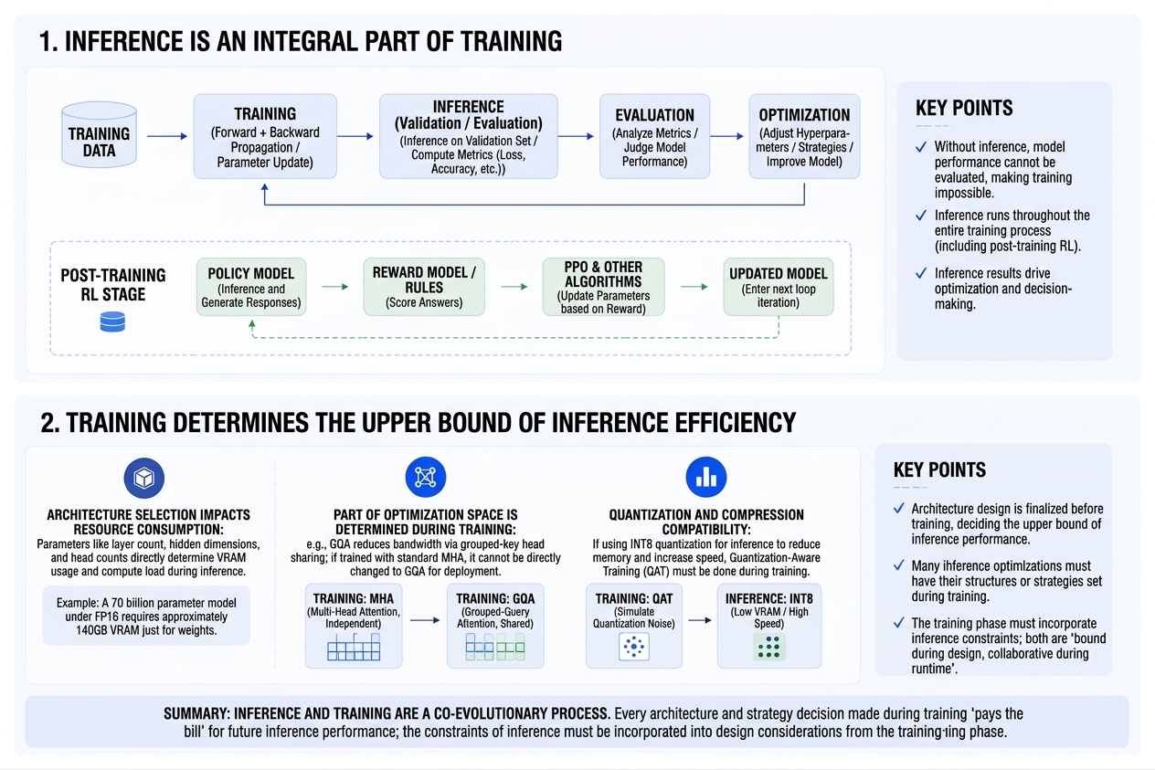
Figure 2. Training and inference cooperation

1. Inference is part of training

Training is not simply "feeding data and updating parameters." It is a continuous training -> inference -> evaluation -> optimization loop:

• After each epoch, the model runs inference on a validation set to calculate metrics such as accuracy and loss and assess the training result.
• During post-training RL, the policy model first generates an answer. An external reward model or a set of rules scores the answer, and an algorithm such as PPO updates the parameters based on that reward.

In other words, without inference we could not know how well the model has learned, and effective training would not be possible.

2. Training determines the upper bound of inference efficiency

The model architecture is chosen before training begins, and these choices directly determine inference performance at deployment time:

• Architecture choices affect resource consumption: the number of transformer layers, hidden dimension, and other architectural parameters directly determine inference memory usage and computation. For example, a 70B-parameter model requires about 140 GB just for FP16 weights, a hard constraint imposed by the architecture.
• Some optimization opportunities must be created during training: certain inference optimizations require the structure to be fixed during training. For example, GQA reduces bandwidth by sharing KV heads in groups. If the model was trained with standard MHA, it cannot simply be changed to GQA at deployment.
• Quantization and compression compatibility: if inference will use INT8 quantization to reduce memory and increase speed, it is preferable to perform quantization-aware training (QAT). We specify the number of quantization bits and simulate quantization noise during the forward pass so that parameters adapt to quantization error. Quantizing directly without QAT can cause substantial accuracy loss and hurt final inference performance.

Inference is not something that happens only after training; it is a collaborative process throughout the entire life cycle. Every architectural decision made during training carries a future inference-performance cost. Inference constraints must therefore be considered during training design. The relationship is bound at design time and collaborative at runtime.

4 Prefill and Decode

Once a trained LLM performs inference, the process from the input prompt to the step-by-step generation of output tokens consists of two key stages: Prefill and Decode. Their computation patterns are fundamentally different. Understanding their characteristics is a prerequisite for targeted inference optimization.

4.1 A Token's Life Cycle

The basic life cycle from receiving a user request to returning a complete response can be summarized as follows:

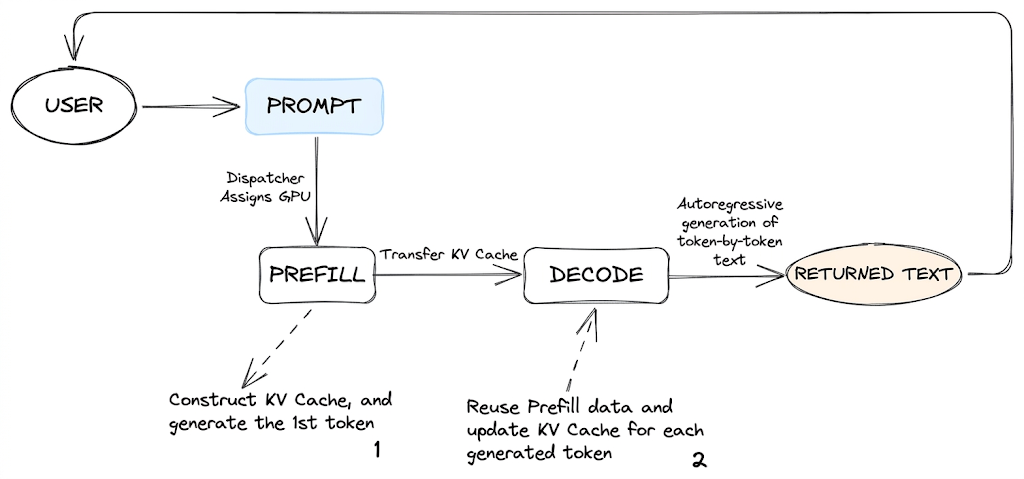
Figure 3. A token's life cycle

• Request scheduling: the user submits a prompt composed of multiple tokens. The inference engine's scheduler, such as the SGLang scheduler, assigns the request to an available GPU or GPU group.
• Prefill stage: the engine performs one computation over the entire assigned prompt. The model processes all input tokens in parallel, builds the complete KV cache, and samples the first output token. This stage has high computational cost and high parallelism.
• Decode stage: autoregressive generation begins. Each step takes only the previously generated token as input, performs a forward pass using the existing KV cache, generates the next token, and appends the new token's KV to the cache. This repeats until an end-of-sequence token (EOS) is produced or the maximum generation length is reached. The computation per step is small, but the growing KV cache must be accessed frequently.
• Return output: the generated token IDs are decoded into text and returned to the user.

Based on this flow, we can examine the underlying computation of Prefill and Decode in more detail.

Note: Techniques that reduce repeated computation, such as prefix caching, are later optimizations rather than required steps in the basic life cycle, so they are not included above.

---

4.2 Prefill

The Prefill stage performs one complete forward pass over the prompt currently scheduled (either a single request or a batch of packed requests). The model processes all input tokens in parallel, builds and writes the initial KV cache, and produces the logits for the first generated token. Consider Prefill for LLaMA-7B:

• Two user requests, with a total of N = 3000 tokens.
• Model config: $L=32$ layers, hidden dimension $d=4096$ , FFN intermediate dimension approximately $\frac{8}{3}d=10923$ , and $\text{heads}=32$ attention heads.

1. FLOPs estimate for one complete forward pass over one batch

The main computations in one forward pass are:

• QKV + Output Projection 4 linear layers, totaling $2\times 4\times N{d}^2=8N{d}^2$
• FFN 2 up-projection layers + 1 down-projection layer, totaling $2\times 3\times (\frac{8}{3}d\times Nd)=16N{d}^2$
• Attention Core Computation  $Q{K}^{\mathrm{\top }}$ and $\mathrm{score}\times V$, totaling $2\times 2\times N^{2}d=4N^{2}d$ .

The total for one layer is $24N{d}^2+4N^{2}d$, and for the entire model $\text{Total FLOPs}\approx L\times (24N{d}^2+4N^{2}d)$. Substituting the values, the computation per layer is:

• Linear projections + FFN (dominant term): $24\times 3000\times {4096}^2\approx 1.21\times {10}^{12}\mathrm{FLOPs}/\mathrm{layer}$.
• Attention term (producing N output tokens): $4\times {3000}^2\times 4096\approx 1.47\times {10}^{11}\mathrm{FLOPs}/\mathrm{layer}$.

Total for 32 layers = 32 x (linear projections + FFN + attention) ≈ 43.4 TFLOPs. In more intuitive terms, this is roughly the work an A100 (312 TFLOPS peak) would perform at full theoretical utilization in 0.14 s, although actual utilization cannot reach 100%.

2. Comparison across prompt lengths

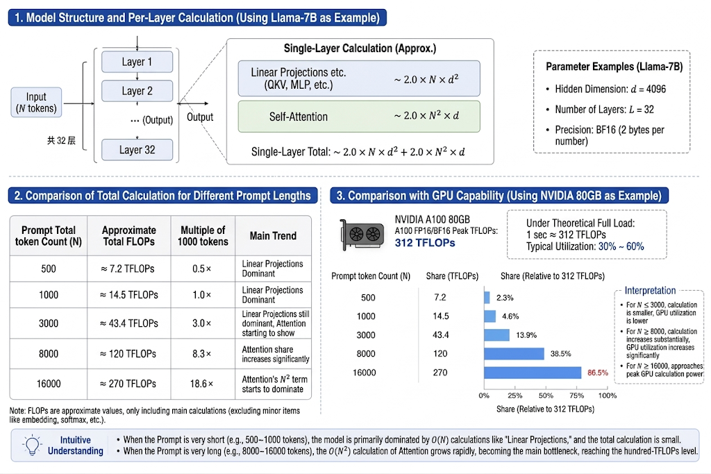
Figure 4. FLOPs comparison for different prompt lengths

At medium lengths (a few thousand tokens), computation grows approximately linearly with $N$. When the prompt becomes very long, the quadratic attention term makes computation increase more rapidly.

3. Memory traffic

Assume the LLaMA-7B weights use FP16 and occupy approximately 14 GB. During Prefill, memory traffic mainly consists of:

• Reading model weights: 14 GB.
• Writing the KV cache: each token (2 bytes per element) requires $2\text{ (KV)}\times 32\text{ layers}\times 4096\times 2\mathrm{byte}\approx 0.5\text{MB}$ of KV-cache space. Processing 3000 input tokens therefore writes approximately 1.5 GB.
• Activations: relatively small and can be ignored.

The total memory traffic in Prefill is therefore approximately 15-16 GB. Combined with the 43.4 TFLOPs computed above, this means that thousands of floating-point operations are performed, on average, for every byte read from GPU memory.

---

The analysis above gives us the following picture:

• Prefill performs a large amount of computation, which increases significantly with prompt length.
• The model weights need to be loaded only once to serve the forward computation for many tokens.

As a result, the GPU's compute units can be used efficiently and arithmetic intensity is relatively high.

4.3 Decode

After Prefill, the LLM enters Decode and generates subsequent tokens one at a time using the accumulated KV cache. Again consider LLaMA-7B, with a 3000-token input prompt (corresponding to a 1.5 GB KV cache) and 2 bytes per token element.

1. FLOPs estimate for one complete forward step over one batch

Similarly, the FLOPs required to generate one token during Decode are:

$$\text{FLOP per token}\approx L\times (24d^2+4Sd)$$

Here, $S$ is the current sequence length, i.e., the number of historical tokens to attend to. For the first output token ($S=3000$):

• Linear projections + FFN: $24\times {4096}^2\approx 4.0\times {10}^8\text{ FLOPs/layer}$.
• Attention: $4\times 3000\times 4096\approx 4.9\times {10}^7\text{ FLOPs/layer}$.

Total computation for 32 layers = Linear Projection + FFN + Attention ≈ 14.4 GFLOPs. Based on the peak computational performance of an A100 40GB, the theoretical computation time is only approximately 0.05 ms. However, the actual latency is far higher than this value, and more importantly, memory consumption is the bigger bottleneck.

2. Memory traffic and bottleneck analysis

Each generated token in Decode requires:

• Reading model weights: 14 GB (all weights must be read for every forward pass).
• Reading the KV cache: 1.5 GB (the initial size when $S=3000$).
• Writing the KV for one new token: approximately 0.5 MB.
• Activations: relatively small and can be ignored.

Total memory traffic is approximately 15.5 GB (combined reads and writes; the 0.5 MB write is negligible). An A100 provides HBM bandwidth of 1.6 TB/s, so the theoretical minimum time to read 15.5 GB is $\frac{15.5\text{ GB}}{1600\text{ GB/s}}\approx 9.7\text{ ms}$. Compared with the theoretical compute time, the GPU spends almost all of its time waiting for data movement.

3. KV-cache accumulation

The KV cache continues to grow as Decode generates a longer response:

• After generating the first token: 1.5 GB + 0.5 MB ≈ 1.5 GB.
• After generating 100 tokens: 1.5 GB + 50 MB ≈ 1.55 GB.
• After generating 2000 tokens: 1.5 GB + 1000 MB ≈ 2.5 GB.

The central issue is that in long conversations or large-batch workloads, every new token requires reading a larger KV cache, further increasing memory traffic and bandwidth pressure. This is why inference engines such as SGLang introduce optimizations including KV-cache reuse and quantization/compression.

---

Decode performs far fewer floating-point operations than Prefill in the same scenario, but every generated token requires reading the complete model weights and a continuously growing KV cache, resulting in extremely low arithmetic intensity. The speed bottleneck is mainly memory bandwidth, while the capacity bottleneck comes from the continued accumulation of the KV cache.

5 Identifying Inference Bottlenecks

In LLM inference, almost all core kernels are determined by the model's computational architecture. Performance is mainly constrained by two factors: data-movement efficiency and compute throughput. The former depends on system bandwidth, namely how much data can be read from or written to memory per second. The latter depends on the compute capability of units such as a GPU's Tensor Cores, namely how many floating-point operations they can complete per second.

5.1 Roofline Model Principles

The Roofline model provides a visual way to identify bottlenecks in inference. By combining theoretical hardware limits with workload characteristics, it helps determine whether an LLM computation is limited by memory bandwidth (memory-bound) or by computation (compute-bound). The axes of a Roofline plot are:

• Horizontal axis: arithmetic intensity (AI), in FLOP/Byte, representing how many floating-point operations can be performed for each byte moved.
• Vertical axis: performance, in FLOP/s, representing the actual number of floating-point operations completed per second. This value can never exceed the hardware's peak compute rate.

The two key quantities are the ridge point and arithmetic intensity.

1. Ridge point: the boundary between compute-bound and memory-bound

$$\text{Ridge point}=\frac{\text{Peak compute (FLOP/s)}}{\text{Memory bandwidth (Byte/s)}}$$

• Physical meaning: at this critical arithmetic intensity, compute capability and memory bandwidth are exactly balanced. The diagram below illustrates the structure of the Roofline model.

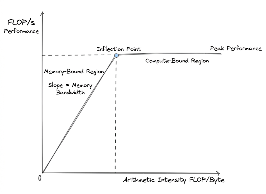
Figure 5. Roofline model

• Decision rule: the ridge point divides the Roofline plot into two regions. The left side is memory-bound, and the right side is compute-bound.

2. Arithmetic intensity: a measure of workload characteristics

$$\text{AI}=\frac{\text{Total floating-point operations (FLOPs)}}{\text{Total memory traffic (Bytes)}}$$

• Calculation: total floating-point operations count all operations required to complete the task, including multiplications and additions; total memory traffic counts all data read from and written to memory, including inputs, outputs, weights, and intermediate results.

Note: memory traffic here means data actually transferred from DRAM; cache hits are excluded.

• Decision rule: compare the calculated AI with the ridge point:

  • AI < ridge point: actual performance ≈ AI × memory bandwidth. The compute units wait for data, and most time is spent on memory reads and writes.
  • AI ≥ ridge point: actual performance ≈ peak compute. Memory supplies data fast enough for the compute units to operate near full capacity.

Compute-bound vs. memory-bound

• Compute-bound: AI is sufficiently high. Compute units are saturated, so performance is primarily determined by peak compute; memory is no longer the bottleneck.
• Memory-bound: AI is low. The processor spends most of its time waiting for data, performance is determined by memory bandwidth x AI, and compute-unit utilization is low.

This is the root cause of the difference between Prefill and Decode in LLM inference.

After identifying the likely bottleneck, we can apply the following procedure:

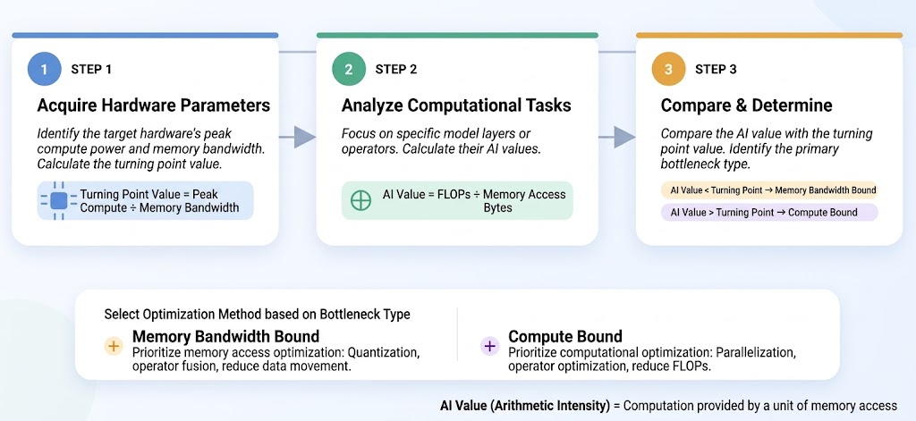
Figure 6. Using the Roofline model to locate inference optimizations

Step 1: obtain hardware parameters. Look up the target hardware's peak compute rate and memory bandwidth, then calculate the ridge point.

Step 2: analyze the workload. Calculate its AI for the specific model layer or operator.

Step 3: compare and decide. Compare AI with the ridge point, then choose an optimization method based on the bottleneck type.

The following examples demonstrate how to use the Roofline model to determine whether LLM inference is compute-bound or memory-bound.

5.2 Roofline Model Example

The core computation in LLM inference is almost entirely matrix multiplication (GEMM). QKV projections and attention-score computation in Attention, as well as the linear transformations in the FFN, all reduce to GEMM operations. To use the Roofline model to identify the bottleneck, we first start with the basic GEMM, derive its arithmetic intensity, and see how matrix dimensions determine the compute and memory-access bottlenecks.

After analyzing GEMM's AI, we return to the two inference stages discussed in Section 2.3 and calculate and compare the AI and ridge point for Prefill and Decode. This answers two key questions:

• Prefill: Why is AI relatively high, and why can a suitable batch size bring it close to or into the compute-bound region?
• Decode: Why is AI extremely low, and why does it remain memory-bound?

---

Arithmetic-intensity analysis of GEMM

Suppose matrices A and B have shapes $M\times K$ and $K\times N$, respectively, and compute $C=A\times B$, producing an $M\times N$ result. For bf16 (2 bytes per element), analyze the computation and data movement:

1. Floating-point operations

$$\text{FLOPs}=2\times M\times K\times N$$

The result matrix C contains $M\times N$ elements. Each element $C_{ij}$ is computed as $\sum _{k=1}^K{A}_{ik}\times B_{kj}$, which contains $K$ multiplications and $K-1$ additions, or approximately $2K$ floating-point operations.

Note: for the same workload, the FLOP count is identical across data types.

2. Data movement

$\text{Bytes}=(M\times K+K\times N+M\times N)\times 2$

The data moved is:

• Read matrix A: $M\times K$ elements.
• Read matrix B: $K\times N$ elements.
• Write result C: $M\times N$ elements.

3. AI

$$\text{AI}=\frac{\text{FLOPs}}{\text{Bytes}}=\frac{2MKN}{(MK+KN+MN)\times 2}=\frac{MKN}{MK+KN+MN}$$

AI increases as the matrix dimensions grow. Larger matrices reuse moved data more effectively, making it easier to reach or exceed the ridge point and become compute-bound.

---

Bottleneck analysis for Prefill and Decode

For the difference in AI between Prefill and Decode discussed in Section 2.3 (higher for the former and lower for the latter), this section uses the same notation and model architecture to analyze their bottleneck types, assuming a batch size of 1.

Notation

• $N$: input sequence length (the number of tokens processed in Prefill).
• $S$: generated sequence length (the KV-cache length in Decode).
• $d$: model hidden dimension.
• $L$: number of transformer layers.
• Data type: bf16.

1. Data-movement analysis

Three components must be considered when calculating data movement:

(1) Model weights: every forward pass reads all parameters from memory (linear layers, LayerNorm, and so on).

(2) Activations: token embeddings and intermediate results from each layer.

(3) KV cache (Decode only): historical tokens' KV values used for Attention.

Prefill stage (processing N tokens in one pass):

$${\text{Bytes}}_{\text{prefill}}=L\times (12d^2+2Nd)\times 2$$

• Total weight per layer: $(4+8)d^2=12d^2$.
• QKV and output projections: each has shape $d\times d$; three reads for QKV plus one output projection read, for $4d^2$ parameters in total.
• FFN layers: two linear layers of shapes $d\times 4d$ and $4d\times d$, for $8d^2$ parameters in total.
• Input + output: $N\times d$ (input) + $N\times d$ (output) = $2Nd$.

Decode stage (generating one token):

$${\text{Bytes}}_{\text{decode}}=L\times (12d^2+2d+2Sd)\times 2$$

• Weight movement: the same as Prefill; all $12d^2$ weights must still be read.
• Input + output: $1\times d$ (input) + $1\times d$ (output) = $2d$.
• KV-cache reads: Attention reads the KV values of the previous $S$ tokens, or $2\times S\times d$.

2. Arithmetic intensity

Here we consider a batch size of 1.

• Prefill arithmetic intensity: ${\text{AI}}_{\text{prefill}}=\frac{L(24N{d}^2+4N^{2}d)}{L(12d^2+2Nd)\times 2}=\frac{24N{d}^2+4N^{2}d}{24d^2+4Nd}$.
• Decode arithmetic intensity:$${\text{AI}}_{\text{decode}}=\frac{L(24d^2+4Sd)}{L(12d^2+2d+2Sd)\times 2}=\frac{24d^2+4Sd}{24d^2+4d+4Sd}$$

The comparison shows that:

• Prefill AI grows linearly with input sequence length $N$.
• As $S$ grows, Decode AI approaches a constant near 1 and is nearly independent of sequence length.

3. Bottleneck diagnosis for LLaMA-7B on an A100

Run LLaMA-7B on an A100 G40 with the same model configuration as above and bf16 computation. The ridge point is $\frac{312\times {10}^{12}}{1.6\times {10}^{12}}\approx 195\text{ FLOPs/Byte}$.

Prefill AI, assuming an input sequence length of $N=100$:

$${\text{AI}}_{\text{prefill}}=\frac{24\times 100\times {4096}^2+4\times {100}^2\times 4096}{24\times {4096}^2+4\times 100\times 4096}\approx \frac{4.03\times {10}^{10}+1.6\times {10}^8}{4.03\times {10}^8+1.64\times {10}^6}\approx 100\text{ FLOP/Byte}$$

Decode AI, assuming $S=100$ (100 tokens have already been generated):

$${\text{AI}}_{\text{decode}}=\frac{24\times {4096}^2+4\times 100\times 4096}{24\times {4096}^2+4\times 4096+4\times 100\times 4096}=\frac{4.02\times {10}^8+1.64\times {10}^6}{4.02\times {10}^8+1.64\times {10}^4+1.64\times {10}^6}\approx 1\text{ FLOP/Byte}$$

Analysis:

1. Prefill: it is still memory-bound, but AI is relatively high; increasing batch size or sequence length can move it toward compute-bound.
2. Decode: AI is extremely low and heavily constrained by memory bandwidth. Each generated token requires reading all weights (approximately 14 GB) while performing only a small amount of computation.

Optimization directions: for Prefill, batching, operator fusion, and Tensor Core optimizations; for Decode, quantization (to reduce weight movement) and KV-cache reuse (RadixAttention), among others.

6 Inference in Real-World Scenarios

The previous sections analyzed the performance characteristics of Prefill and Decode theoretically. In real applications, different scenarios amplify different bottlenecks. Two common examples are Agent collaboration and multi-turn conversations; we analyze their inference bottlenecks below.

6.1 Agent Collaboration

Inference performance in collaborative-agent scenarios faces the following challenges:

1. Tool-call overhead

Agentic workflows typically involve repeated tool-call loops: model generation -> tool execution -> result return -> model inference again. Each loop requires a complete Prefill over the accumulated context.

• Repeated Prefill: after every tool call, shared context such as system prompts, conversation history, and tool definitions must be prefilled again.
• Context expansion: tool definitions and execution results quickly increase the input length, so the cost of subsequent Prefill operations continues to rise.

2. Cross-agent communication cost

In a serially executed distributed multi-agent system, message passing and state synchronization between agents introduce network latency and serialization overhead.

• Effect on Prefill: messages passed between agents become part of the next agent's input context, increasing Prefill input length.
• Effect on Decode: if agents must wait for one another's outputs, end-to-end latency increases. When multiple Decode requests compete for resources on the same GPU, network latency further amplifies queueing time.

6.2 Multi-Turn Conversations

The defining characteristic of a multi-turn conversation is that each new request depends on the previous history, causing input length to grow linearly with the number of turns.

1. Linear growth in Prefill latency

Within one conversation window, each turn processes the complete history, so TTFT grows linearly with the number of turns. For a long conversation (more than 10 turns), Prefill can account for most of the total response time. Suppose each turn adds 200 tokens and the model's Prefill speed is 1000 tokens/s: in turn 1, TTFT is approximately 200 ms; in turn 10, TTFT is approximately 2000 ms. As the conversation continues, Prefill response time increases markedly.

2. KV-cache memory usage

Keeping the complete conversation history in the KV cache consumes substantial GPU memory. With long contexts (for example, 100K tokens), it can occupy tens of gigabytes and limit the number of concurrent requests.

• Memory access becomes the bottleneck: with long contexts, reading the KV cache can take longer than the actual computation.
• Batching efficiency declines: large KV caches reduce the number of requests that can be processed concurrently, lowering GPU utilization and overall throughput.

7 Summary and Exercises

7.1 Summary

This chapter analyzed the core mechanisms and performance bottlenecks of LLM inference. Starting from the fundamental differences between training and inference, we examined the computation characteristics of the two key stages, Prefill and Decode, and introduced the Roofline model as a performance-analysis tool. The Agent-collaboration and multi-turn-conversation scenarios illustrated challenges faced by practical inference systems.

7.2 Exercises

1. What are the differences and connections between training and inference?

Hint: consider whether model parameters are updated, the computation process, compute and storage costs, and the relationship between the two.

2. Compare and contrast Prefill and Decode, and analyze the performance bottleneck of each.

Hint: consider how tokens are processed, computation patterns, parallelism, arithmetic intensity, and memory-access patterns.

3. What is the significance of the Roofline model?

Hint: explain the meanings of the horizontal and vertical axes, the peak compute rate and memory bandwidth of the platform, and the ridge point.

4. How can the Roofline model be used to identify an inference bottleneck? Choose a concrete scenario and analyze it.

Hint: clearly describe the hardware parameters, AI calculation, and the complete comparison with the ridge point.

5. In an RAG+LLM application, suppose multiple financial documents form a knowledge base for analyzing economic questions, and users have a long multi-turn conversation in the same window. What are the main performance bottlenecks?

Hint: analyze context growth caused by injecting RAG retrieval results, accumulated multi-turn history, increased Prefill computation, and KV-cache memory usage.

References

• SGLang Documentation
• NVIDIA H100 Tensor Core GPU
• Deploying DeepSeek with PD Disaggregation and Large-Scale Expert Parallelism on 96 H100 GPUs
• Inside NVIDIA Groq 3 LPX: The Low-Latency Inference Accelerator for the NVIDIA Vera Rubin Platform
• Tool Observations Are the Hidden Prefill in Local Agent Loops on RDNA4
• Diy-LLM Chapter 9: Scaling Laws
• Diy-LLM Chapter 10: Inference