Chapter 9 Multi-process and Tensor Parallelism

In the previous chapters, we followed a request through the complete end-to-end processing pipeline and examined paged KV Cache, RadixAttention, and prefix caching. These mechanisms explain how to manage and reuse the KV Cache efficiently, but deployment raises a more fundamental question: if a single GPU does not have enough memory or compute capacity, how can multiple GPUs work together to run the same model?

This chapter addresses that question by first distinguishing the roles of multi-process execution and tensor parallelism, then explaining how GPUs communicate and how weights and computation are partitioned. Finally, it connects these mechanisms into the complete workflow, from loading the model to processing requests.

1 Learning Objectives

After completing this chapter, you should be able to answer the following questions:

• What problems do multi-process execution and tensor parallelism each solve, and why do they need to work together?
• How do ranks keep request processing consistent, and how do they combine their local computation results?
• How are linear layers, vocabulary layers, and the KV Cache partitioned, and what constraints apply?
• How do the processes cooperate when starting the inference engine, loading the model, and processing a request?

2 Multi-process and Tensor Parallelism

Before examining the implementation, we will start with GPU memory requirements to understand when multiple GPUs are needed and what costs they introduce.

2.1 Why Consider Multiple GPUs When the Weights Fit on One GPU?

Take Qwen2.5-32B as an example. Assuming approximately $3.2\times {10}^{10}$ parameters and BF16 precision (2 bytes per parameter), the weights alone require:

$$3.2\times {10}^{10}\times 2\approx 64\mathrm{GB}$$

An A100 80GB GPU can hold these weights, but the context length and concurrency it can support also depend on other GPU memory overhead.

During model inference, GPU memory is also needed for:

• KV Cache: With a fixed model architecture and cache precision, its memory usage grows with the total number of cached tokens. For sequences of equal length, this can be understood as growth proportional to the product of sequence length and batch size.
• Temporary activations, operator workspaces, and communication buffers.
• Capture and execution buffers required when CUDA Graph is enabled.

Therefore, having enough memory for the weights does not mean the model can run reliably under the target workload. A model may work normally with low concurrency and short contexts, yet run out of memory (OOM) when concurrency or context length increases.

If the parameter count grows further to $1.6\times {10}^{12}$ , the BF16 weights alone require approximately $3.2\mathrm{TB}$ , far beyond the capacity of a single GPU.Distributing most of the weights and some intermediate computation across multiple GPUs reduces the memory pressure on each GPU. With a suitable model, workload, and interconnect, it may also reduce the latency of a single forward pass or leave room for a larger batch.

However, using multiple GPUs does not necessarily make computation faster. TP introduces frequent communication and synchronization between GPUs, so its benefits depend on factors such as the amount of computation, batch size, and GPU communication bandwidth.

2.2 How do the two support multi-card parallelism?

Multi-process execution is a way to organize a system: multiple processes, each with its own address space, cooperate through mechanisms such as message passing. To work around the Python GIL and support efficient inference, the system uses a multi-process architecture. Typical components include:

• API Server and Tokenizer process: Receive requests and convert text into tokens.
• Detokenizer process: Converts the model's output tokens back into text.
• Scheduler process: The core scheduling process. Each Scheduler process corresponds to a rank bound to one GPU. It handles request queuing, continuous batching, KV Cache allocation and management, and triggers local computation.
• Engine/TpModelWorker/ModelRunner process: Run inside the Scheduler process and handle the actual model forward pass, weight loading, and communication across ranks.

Note: In this setup, each rank corresponds to one GPU and runs in a separate process.

Tensor Parallelism (TP) is a model parallelism strategy: it partitions **Weights of the same layer、vocabulary ** across multiple ranks, allowing them to jointly compute results for the same batch of inputs. Consider a linear layer:

• On a single GPU, the complete matrix multiplication is $Y=XW$.
• With multiple GPUs, the weight matrix is partitioned by columns (the output dimension) or by rows (the input dimension). Each GPU holds only part of the weights and computes a local result. Where needed, operations such as All-Reduce and All-Gather combine those results into the complete output.

For a given request, every token is computed jointly by the entire TP group. Coordination between processes ensures that all ranks always process the same batch.

Note: mini-SGLang currently supports only TP. SGLang also supports advanced strategies such as Data Parallelism (DP) and Pipeline Parallelism (PP).

In essence, multi-process execution handles process organization, information exchange, and scheduling coordination, while TP partitions computation for parallel execution. Next, we will examine the mechanisms that make both possible.

3 Communication and Partitioning

Distributing the model across multiple GPUs requires satisfying two conditions simultaneously: each rank processes the same input at the same step, and local results can reconstruct the original model computation —— the former relies on scheduling and communication coordination, while the latter is guaranteed by partitioning rules and tensor communication. If the model can fit on a single GPU, no partitioning or cross-rank communication is needed(No data plane), and the complete weights can be loaded directly.

3.1 Communication: Align Tasks First, Then Combine Results

Even with a single rank, inter-process communication is still needed between the API Server, tokenization workers, and Scheduler. When the TP size is greater than 1, coordination of requests between ranks and communication of GPU tensors are also required.

1.Control plane: Ensure that ranks execute corresponding tasks at the same step (execution consistency)

The mini-SGLang implementation discussed in this chapter mainly uses two mechanisms:

• ZeroMQ (ZMQ): Transfers requests, token IDs, sampling parameters, and generation results between the API Server, tokenization and detokenization workers, and the rank 0 Scheduler. With multiple ranks, rank 0 also broadcasts request messages to the other Schedulers through ZMQ's publish/subscribe mechanism.
• Gloo CPU process group: Created through torch.distributed, it is used for startup barriers, broadcasting the NCCL Unique ID during PyNCCL initialization, and synchronizing the number of messages received in each round of non-blocking receives at runtime.

Because ranks may progress at different speeds, allowing every rank to communicate directly with the Tokenizer/Detokenizer can lead to inconsistent message handling. Therefore, only rank 0 handles external communication; the other ranks receive information from rank 0.

2.Data plane: Exchange GPU tensors used in model computation (result correctness)

NCCL is NVIDIA's collective communication library for GPUs, and mini-SGLang's PyNCCL wraps NCCL. The default multi-GPU execution path enables PyNCCL; --disable-pynccl falls back to PyTorch's NCCL backend. Two common operations are:

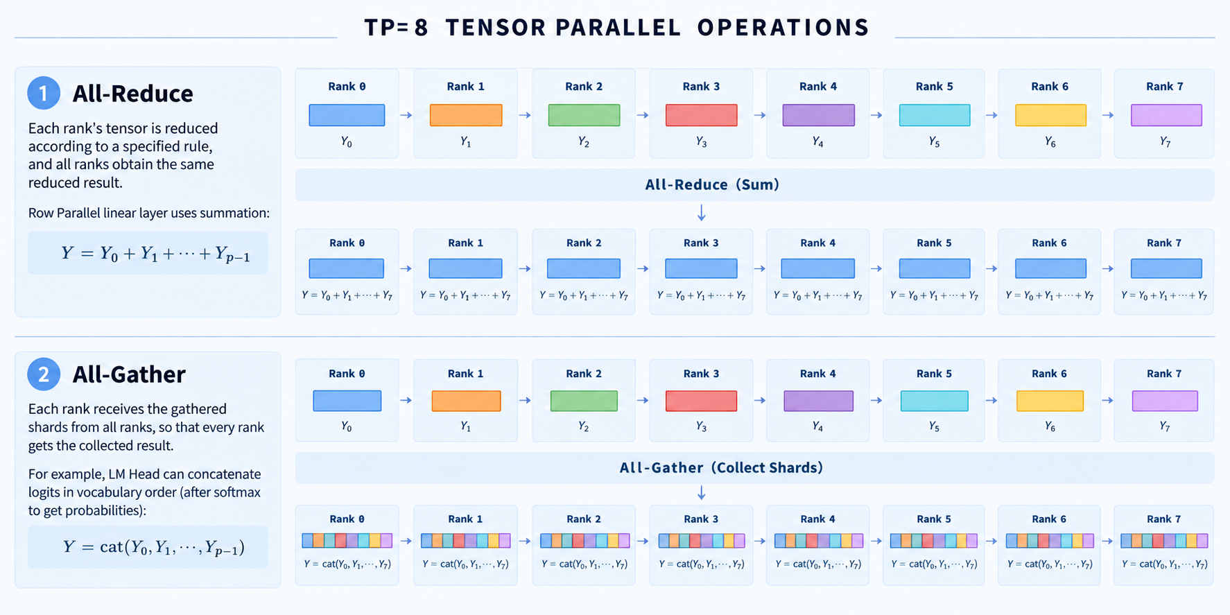
Figure 1. Example of data exchange for TP=8

• All-Reduce: Reduces tensors from all ranks according to a specified operation and makes the reduced result available to every rank. Row-parallel linear layers use summation:

  $$Y=Y_0+Y_1+\cdots +Y_{p-1}$$

• All-Gather: Collects tensor shards from all ranks and makes the gathered result available to every rank. For example, the LM Head can use it to concatenate logits in vocabulary order; applying softmax to the logits then produces probabilities:

  $$Y=\mathrm{cat}(Y_0,Y_1,\dots ,Y_{p-1})$$

If the required collective communication across ranks is missing—for example, after certain row-parallel linear layers or when producing the final vocabulary output—subsequent computation will receive values that do not match the original model's results, causing severe errors in the final output.

Put simply, the control plane ensures that all ranks work on the same task, while the data plane ensures that their results combine correctly. Both are essential. Before the LLM can process requests, model weights, the vocabulary, and configuration information must also be loaded correctly. The next section explains how these are partitioned and loaded across ranks.

3.2 Partitioning

In an LLM inference engine, the core goal of partitioning is to distribute model weights and computation across multiple GPUs so that a large model fits in GPU memory, while improving throughput through parallel computation.

Multi-GPU partitioning must strictly follow mathematical equivalence. What needs to be partitioned and what should remain intact generally follows these principles:

• Replication of retained parts: Components such as RMSNorm that require synchronization for every segment are fully replicated on each rank.
• Dimension-wise partitioning: Weight matrices and their corresponding biases are evenly split along the output (row) dimension by tp_size.

The partitioning methods are illustrated below:

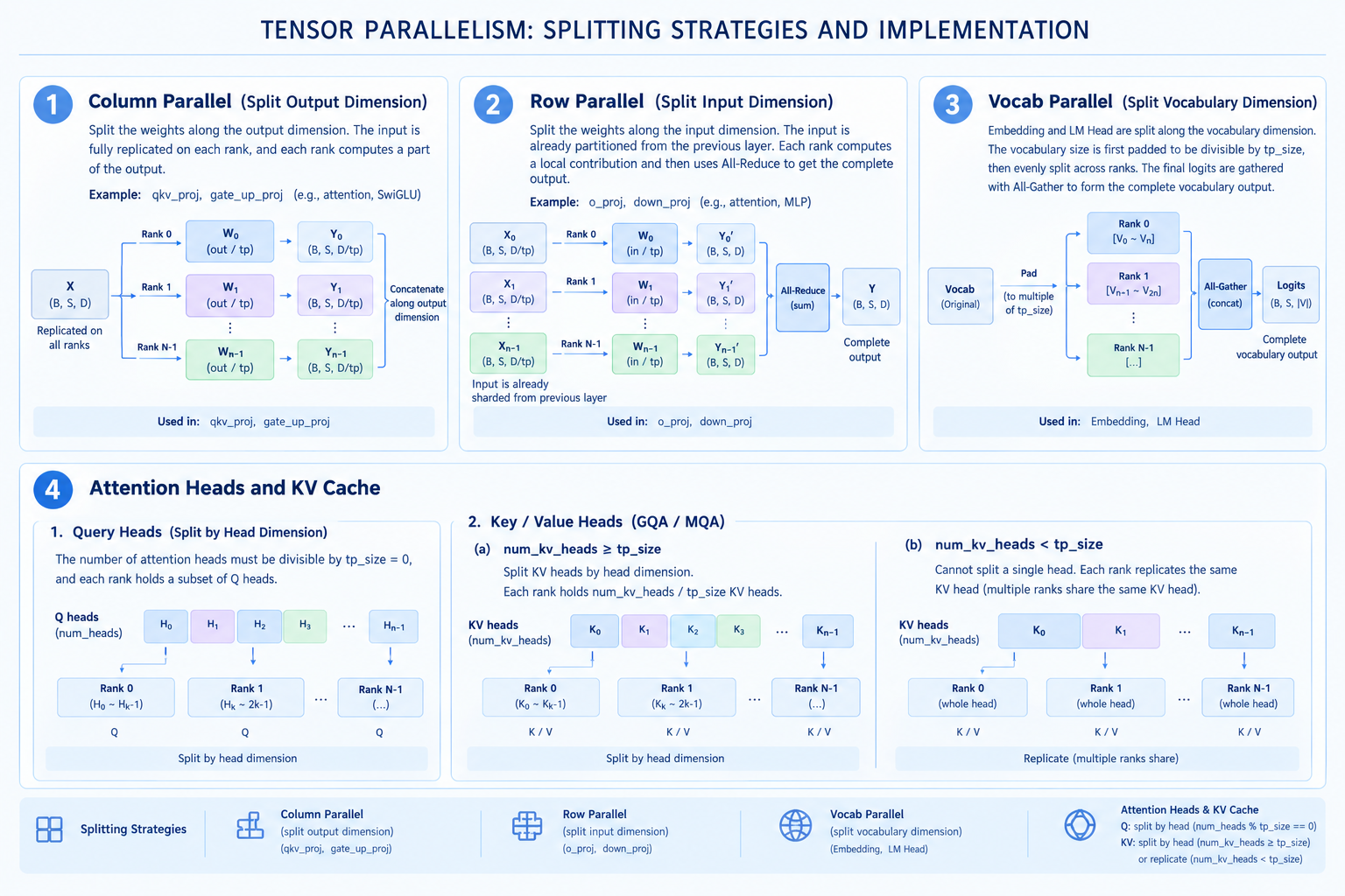
Figure 2. Sharded loading methods

• Column Parallel (partition along the output dimension): The weights are partitioned along the output dimension, and the complete input is replicated on every rank. Each rank computes part of the output. Examples include qkv_proj in attention and gate_up_proj in SwiGLU.
• Row Parallel (partition along the input dimension): The weights are partitioned along the input dimension. The input is already a local shard produced by the preceding layer. Each rank computes a local contribution, and All-Reduce sums these contributions to obtain the complete output. Examples include o_proj in attention and down_proj in the MLP.
• Vocab Parallel (partition along the vocabulary dimension): The Embedding and LM Head are partitioned along the vocabulary dimension. The vocabulary size is first padded to be divisible by tp_size, then divided evenly across ranks. The final logits are concatenated through All-Gather to produce the complete vocabulary output.
• Attention heads and KV Cache:
  • Query heads: These are almost always partitioned along the head dimension, requiring num_attention_heads % tp_size == 0. Each rank holds only a subset of the Q heads.
  • Key/Value heads: If num_kv_heads >= tp_size, the heads are partitioned along the head dimension, with each rank holding num_kv_heads//tp_size KV heads. If num_kv_heads < tp_size, an individual head cannot be partitioned further in this scheme, so KV heads are replicated, with multiple ranks holding copies of the same head.

Partitioning targets large weights; small layers are usually retained in full. When choosing tp_size, consider both:

1. The model's parameter count and the memory capacity of each GPU.
2. Architectural constraints, such as the number of heads, and the computation scheme, so that combining local results remains mathematically equivalent to the complete computation.

4 From Startup to Execution

The user only needs to run a launch command specifying the model path and optional parameters such as the TP size; the system then handles the remaining work automatically. The entry point is launch_server. After parsing the arguments, the main process enters run_api_server, which starts the subprocesses, waits for them to become ready, and then serves requests.

Step 1 start_subprocess starts the subprocesses according to the configuration:

• A number of Scheduler processes equal to the TP size (tp_info.size). The parent process assigns each subprocess its own DistributedInfo(rank, world_size). Process names follow a pattern such as minisgl-TP{i}-scheduler.
• One Detokenizer process.
• num_tokenizer Tokenizer processes. With the default num_tokenizer=0, a shared worker handles both tokenization and detokenization, and no separate Tokenizer process is started.

The main process waits for readiness acknowledgments through ack_queue: one from the rank 0 Scheduler, one from each Tokenizer, and one from the Detokenizer.

Step 2 Inside each Scheduler process, initialization in _run_scheduler proceeds as follows:

• A Scheduler is created, which in turn creates an Engine.
• The Engine binds to the GPU corresponding to the current rank, initializes distributed communication, loads and partitions weights according to the TP rules, initializes the KV Cache and Attention Backend, performs CUDA Graph capture, and completes other initialization work.
• The Scheduler then initializes managers for Table, Cache, Prefill, and related functionality, along with ZMQ-based message sending and receiving. After all ranks synchronize through sync_all_ranks(), they enter scheduler.run_forever() to wait for and process requests.

Step 3 Once all subprocesses are ready, the API Server in the main process starts listening on the specified port and provides an OpenAI-compatible API to receive requests. The complete request-processing path was covered in Chapter 2: The Journey of a Request, so it is not repeated here.

5 Summary and Exercises

5.1 Summary

This chapter introduced the factors to consider before deploying an open-source model and starting an inference service on one or more GPUs, including how many GPUs to use for a model. It then explained how TP partitions and loads weights and how multiple processes cooperate to handle requests. TP is only one way to parallelize model weights; the SGLang source code contains other parallelism and communication implementations that can be read for comparison.

5.2 Exercises

1. What problems do multi-process execution and TP each solve?
2. Why can't each rank independently receive an arbitrary number of requests? What information must remain consistent during processing, and how are consistency and correctness ensured?
3. Why does doubling the TP size not necessarily halve GPU memory usage or double inference speed? Explain in terms of replication overhead, the number of KV heads, and communication costs.

References

• Chapter 2: The Journey of a Request
• mini-SGLang
• SGLang
• Qwen2.5-32B Configuration