强化学习与控制
On this page
5. Temporal-Difference Methods
Temporal-difference (TD) methods combine ideas from Monte Carlo methods and dynamic programming. They update estimates at each step without waiting for an episode to finish.
For unfamiliar symbols, consult the terms and formulas quick reference. Expand the plain-language explanations beside this chapter's formulas without leaving the page.
Embodied AI perspective: TD learning is the core update mechanism behind many modern deep RL algorithms, including DQN's Q updates and DDPG/SAC's Critic updates. It lets a robot learn incrementally while interacting with its environment.
This chapter follows the MDP reward-index convention: executing r and reward also denote the reward from this transition.
5.1 Temporal-difference estimation
Recall the Monte Carlo update in
The complete return
Monte Carlo estimation can update values incrementally across episodes, but it must first wait for an episode to finish to obtain its complete return. This can make learning slow for long episodes and unsuitable for tasks without a clear endpoint.
Temporal-difference (TD) estimation instead combines the immediate reward with the estimated value of the next state:
In plain language: what does one TD update calculate?
Suppose the old estimate is
- Calculate the target:
, the immediate reward plus an estimate of the future. - Calculate the error:
. This target is above the old estimate. - Move partway toward it:
.
Quick reference: bootstrapping, TD error, and learning rate.
The quantity
Updating an estimate using another current estimate is called bootstrapping. TD combines Monte Carlo's ability to learn without transition probabilities with dynamic programming's use of existing value estimates. It can therefore update before a complete return is available.
If executing
5.2 A numerical example
Consider the
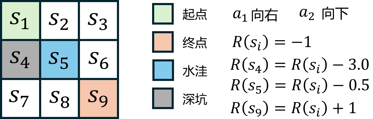
Each step incurs reward
The following Python example compares TD and Monte Carlo estimation:
import random
from collections import defaultdict
import numpy as np
import pandas as pd
import matplotlib.pyplot as plt
import time

# ---------- Parameters ----------
gamma = 0.9
alpha = 0.1            # Learning rate (try 0.05–0.2)
episodes = 100000
states = [f"s{i}" for i in range(1, 10)]
terminal = "s9"
start = "s1"

coords = {
    "s1": (0,0), "s2": (0,1), "s3": (0,2),
    "s4": (1,0), "s5": (1,1), "s6": (1,2),
    "s7": (2,0), "s8": (2,1), "s9": (2,2)
}

# ---------- Environment ----------
def legal_actions(s):
    r, c = coords[s]
    acts = []
    if c < 2: acts.append("right")
    if r < 2: acts.append("down")
    return acts

def step(s, a):
    r, c = coords[s]
    if a == "right": r2, c2 = r, c + 1
    elif a == "down": r2, c2 = r + 1, c
    s2 = [k for k, v in coords.items() if v == (r2, c2)][0]
    reward = -1.0
    if s2 == "s4": reward -= 3.0     # Pit
    if s2 == "s5": reward -= 0.5     # Puddle
    if s2 == "s9": reward += 1.0     # Goal +1 gives net reward 0
    done = (s2 == terminal)
    return s2, reward, done

def policy(s):
    acts = legal_actions(s)
    return random.choice(acts)

def generate_episode():
    episode = []
    s = start
    while True:
        if s == terminal:
            episode.append((s, None, 0))
            break
        a = policy(s)
        s2, r, done = step(s, a)
        episode.append((s, a, r))
        s = s2
    return episode

# ---------- First-Visit Monte Carlo ----------
def first_visit_mc(num_episodes=episodes, gamma=0.9):
    V = defaultdict(float)
    N = defaultdict(int)
    for _ in range(num_episodes):
        episode = generate_episode()
        G = 0
        visited = set()
        for s, a, r in reversed(episode):
            G = gamma * G + r
            if s not in visited:
                visited.add(s)
                N[s] += 1
                V[s] += (G - V[s]) / N[s]
    return V

# ---------- TD(0) prediction ----------
def td0_value_prediction(episodes=episodes, alpha=alpha, gamma=gamma, start="s1"):
    V = defaultdict(float)  # Initialize all values to 0
    for _ in range(episodes):
        s = start
        while s != terminal:
            a = policy(s)
            s2, r, done = step(s, a)
            # TD(0) update
            V[s] += alpha * (r + gamma * V[s2] - V[s])
            s = s2
    return V

s_t = time.time()
V_mc = first_visit_mc()
t_cost_mc = time.time() - s_t
print(f"First-Visit MC time: {t_cost_mc:.2f} seconds")

# ---------- Print results ----------
grid_mc = np.array([[V_mc[f"s{r*3+c+1}"] for c in range(3)] for r in range(3)])
df_mc = pd.DataFrame(grid_mc.round(3),
                     columns=["col1","col2","col3"],
                     index=["row1","row2","row3"])
print(df_mc)

s_t = time.time()
V_td0 = td0_value_prediction()
t_cost_td0 = time.time() - s_t

print(f"TD(0) time: {t_cost_td0:.2f} seconds")

grid_td0 = np.array([[V_td0[f"s{r*3+c+1}"] for c in range(3)] for r in range(3)])
df_td0 = pd.DataFrame(grid_td0.round(3),
                      columns=["col1","col2","col3"],
                      index=["row1","row2","row3"])
print(df_td0)
An example output is:
First-Visit MC time: 0.57 seconds
      col1   col2  col3
row1 -4.43 -2.149  -1.0
row2 -2.15 -1.000   0.0
row3 -1.00  0.000   0.0
TD(0) time: 0.47 seconds
       col1   col2  col3
row1 -4.110 -2.216  -1.0
row2 -2.182 -1.000   0.0
row3 -1.000  0.000   0.0
Both methods produce similar values in this example, with TD taking slightly less time. TD updates during an episode, which can improve learning efficiency when complete episodes are expensive to collect. Values and runtimes vary between runs.
5.3 Deriving the TD target
Where does
Under the expectation for a given policy, the complete return can be replaced by an immediate reward plus the discounted next-state value. This motivates the sampled approximation:
Step by step: why is this an approximation, not an equality?
The recursion
Even the true value is an average return. Suppose the next state's subsequent return is either
Quick reference: Bellman equation and expectation.
Substituting this target into the Monte Carlo update gives the TD update. The relation is about expectations, not equality between an individual sampled target and a complete return. A stable policy, sufficient exploration, and repeated updates are important for value estimation. As
Insufficient coverage or too few updates can leave estimates unstable. Converging value estimates is also different from finding an optimal policy: prediction evaluates a given policy; control additionally improves it. Before values have converged, the bootstrap term is itself approximate. Learning rates, exploration settings, alternative TD targets, and function approximators all affect practical training behavior.
5.4 n-step temporal difference
The target
The first term is the discounted sum of
The limiting cases connect TD and Monte Carlo:
For an episodic task, collecting rewards through termination gives the complete Monte Carlo return. Smaller
5.5 Comparing dynamic programming, Monte Carlo, and TD
| Method | Environment model | Update timing | Estimation | Main tradeoffs |
|---|---|---|---|---|
| Dynamic programming | Required | During value-update sweeps | Bootstrapping | Can converge quickly, but requires a complete environment model |
| Monte Carlo | Not required | After an episode | Sampling | Unbiased complete-return samples for a fixed policy; requires full episodes and often has high variance |
| Temporal difference | Not required | Each interaction step | Sampling and bootstrapping | Timely, efficient updates with lower variance; bootstrap bias and sensitivity to exploration and learning settings |
5.6 Sarsa
Sarsa is an on-policy TD control algorithm for estimating
5.6.1 TD estimation of action values
The action-value update is analogous to the state-value update:
5.6.2 Sarsa procedure
Combining the control loop with TD action-value estimation gives the following procedure. See the practice material for complete implementations.
- Initialize
. Reset the environment to for each episode and select using an -greedy policy. - Starting at
, execute and observe and . - If
is terminal, update toward and end the episode. - Otherwise, select
in using the same policy. Update toward . - Set
and repeat steps 2–4, executing the action already selected.
Sarsa updates without waiting for episode completion, using
5.6.3 Exploration policy
Sufficient exploration is important for learning values. Sarsa commonly uses an
The exploration rate
5.7 Q-learning
Q-learning is an off-policy TD control algorithm. Instead of evaluating the action actually selected at the next state, it uses the highest estimated next-state action value. This lets it learn a greedy target policy while collecting experience with a different behavior policy:
In plain language: how does Q-learning's max differ from Sarsa?
Suppose the next state has two actions with estimates
- Sarsa uses the selected action, giving target
. - Q-learning uses the highest estimated value, giving target
.
Here
Quick reference: on-policy and off-policy, max and argmax.
The procedure is as follows. See the practice material for complete implementations.
- Initialize
and reset the environment to for each episode. - Starting at
, choose and execute using a behavior policy such as -greedy. Observe and . - If
is terminal, update toward and end the episode. Otherwise, update toward . - Set
and repeat steps 2–3. The maximum in the update target does not depend on the action actually selected next.
Q-learning uses
| Q-learning | Sarsa | |
|---|---|---|
| Policy type | Off-policy | On-policy |
| Update target | Best estimated next action | Next action actually selected |
| Learning behavior | Often more aggressive | Accounts for behavior-policy exploration |
| Typical consideration | Learning a greedy policy while exploring | Evaluating the consequences of the policy actually executed |
5.8 On-policy and off-policy learning
The distinction concerns the behavior policy, which collects experience, and the target policy, which is evaluated or improved. If they are the same, learning is on-policy; if they differ, learning is off-policy.
For a driving analogy, an on-policy learner evaluates and improves the driving behavior it currently follows. An off-policy learner may evaluate an idealized driving policy while collecting experience under different behavior dictated by traffic or road conditions.
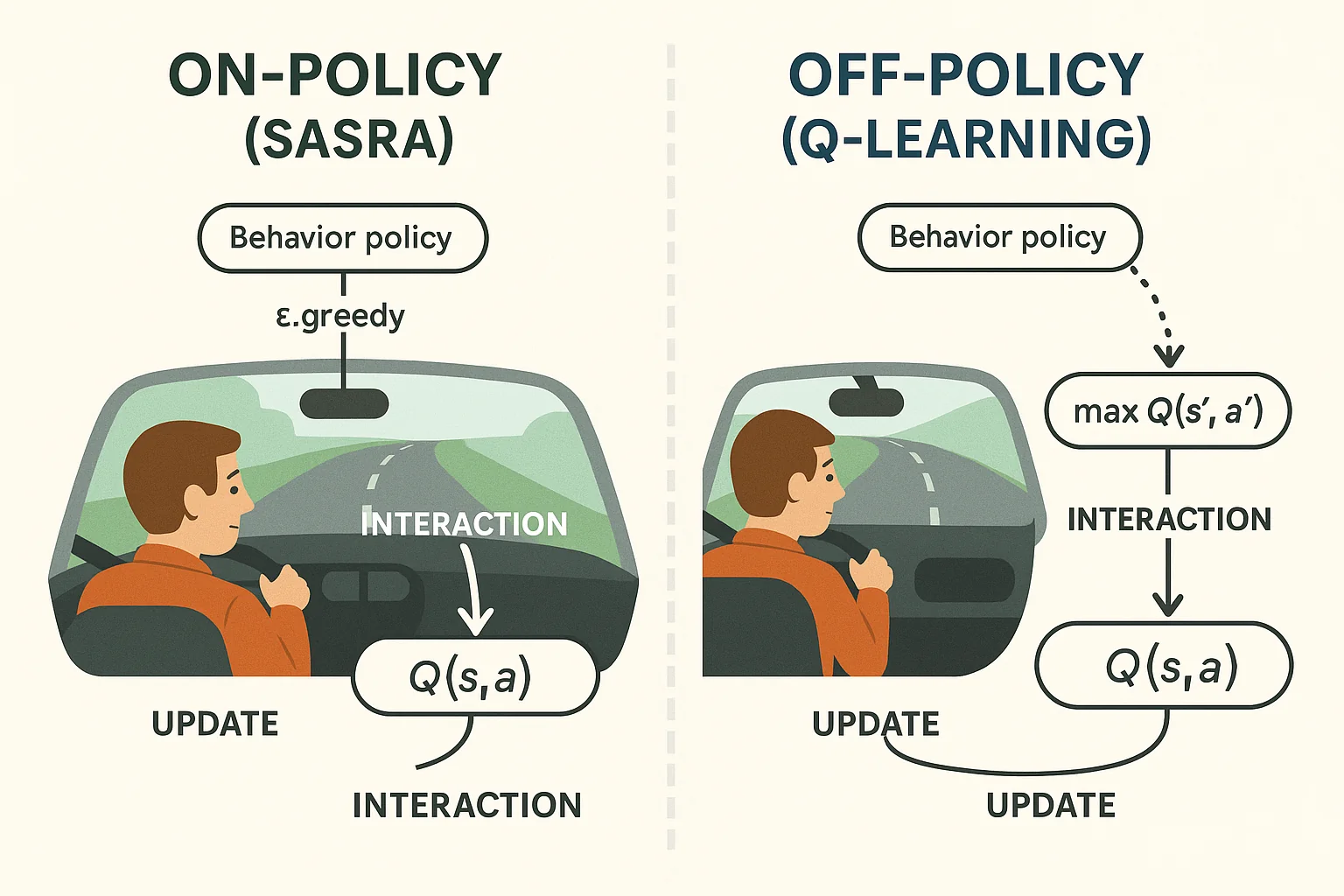
On-policy methods learn directly from their current behavior. Off-policy methods offer more flexibility to reuse data from other behavior policies, but can face additional stability and convergence challenges.
5.9 Questions
Are Monte Carlo and TD methods both model-free?
Yes. They learn values or policies from interaction without requiring an explicit model of the environment's dynamics.
What are their respective strengths and weaknesses?
Monte Carlo methods learn directly from complete returns. For a fixed policy, those returns provide unbiased samples, but updates must wait for full episodes and can have high variance. Long or nonterminating episodes are problematic. TD methods learn during interaction, work with both episodic and continuing tasks, and can use function approximation in large state spaces. Bootstrapping introduces bias, and learning rate and exploration settings affect stability. Choose according to the task and the available experience.
What is Q-value overestimation, and how can it be reduced?
Overestimation occurs when learned state or action values exceed their true values because of sampling noise or properties of the learning algorithm. Double Q-learning separates action selection from evaluation to reduce this effect. Prioritized replay, target networks, and exploration strategies also affect data coverage and training stability, although they serve different roles from the direct overestimation correction in Double Q-learning.
How do on-policy and off-policy methods differ?
On-policy methods collect samples with the policy they are learning about. Off-policy methods can collect data with a different behavior policy and use it to improve their target policy.
Why is exploration necessary?
The optimal policy is initially unknown. Following only currently preferred actions can leave useful states and actions unexplored and miss better strategies. Common exploration mechanisms include