强化学习与控制
On this page
2. Markov Decision Processes
A Markov decision process (MDP) is the core problem model in reinforcement learning. Whether training a quadruped to walk or a robotic arm to grasp, the first step is to identify the state space, action space, transition probabilities, and reward function.
For unfamiliar symbols, consult the terms and formulas quick reference. Expand the plain-language explanations beside this chapter's formulas without leaving the page.
Embodied AI perspective: For robotic grasping, the state
might contain joint angles and object poses, the action might specify joint torques, and the reward might indicate grasp success. Defining these elements makes the task suitable for RL.
2.1 Agent–environment interaction
An agent interacts with its environment over discrete time steps. At step
Chapters 2–6 (MDPs, dynamic programming, Monte Carlo, temporal difference, and DQN) index rewards by the step at which they arrive: executing
Uppercase
The later policy-gradient, Actor-Critic, and SAC chapters retain the convention of indexing rewards by the action that produces them. The sample correspondence is
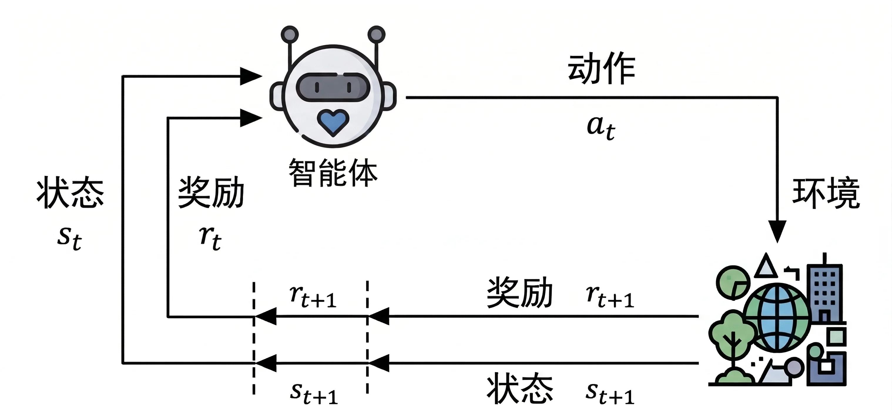
Repeating this interaction produces a trajectory:
A complete trajectory from an initial state to a terminal state is an episode, ending after a finite number of steps
To solve a problem with RL, first specify its state space, action space, transition probabilities, and reward function. An MDP is commonly defined as the tuple:
Here
2.2 The Markov property
The central assumption is the Markov property: the distribution of the next state depends only on the current state and action, not on the earlier history:
In plain language: why does the Markov property only need the present?
The point is that the current state contains enough information, not that the robot must forget the past. A ball's position alone usually cannot tell you where it will move next; including velocity gives you more information. The vertical bar means “given this information.” The equality says that adding the past history does not change the conditional distribution of the next state.
More context: states versus observations.
Real robots typically receive partial observations. For example, a current lidar scan may miss occluded objects. Such problems can be modeled as partially observable Markov decision processes (POMDPs). Stacking past frames can help approximate a Markov state, but does not guarantee recovery of the full state.
2.3 State transition matrices
For a finite state space, a directed graph can show how states connect:
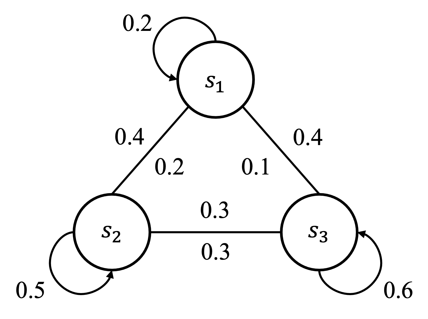
Transition probabilities can be represented as a matrix:
Here
2.4 Objectives and returns
The agent aims to learn a policy whose actions maximize expected cumulative reward. This cumulative quantity is called the return:
The discount factor
For an episode terminating at
A useful measure of the discount factor's reach is the effective horizon:
For
The return has the recursive definition:
Step by step: how does a long reward sum become two terms?
- Keep the first term
, the reward just produced by the current action. - Every remaining term contains at least one factor of
. Factor it out. - What remains in parentheses is exactly the return starting at the next time step,
:
This is just factoring: no future rewards disappear. Check with the two-step example above:
Symbol guide:
2.5 Policies and values
2.5.1 Policy
A policy
Policies may be deterministic, always choosing the same action in a given state, or stochastic, sampling actions from a distribution. Stochastic policies are common in embodied AI because they support exploration and robustness.
2.5.2 State value
The state-value function is the expected return from a state when following policy
In plain language: how do I read the expectation and conditional bar?
Read the formula as: “Starting at state
For example, returns of
Quick reference: expectation and value.
2.5.3 Action value
The action-value function is the expected return given state
2.5.4 Relating state and action values
In plain language: why is V a weighted average of Q?
If the left and right actions have
State value is the policy-weighted average of action values. It evaluates following the policy from a state, while action value evaluates choosing a particular action there.
2.6 Model-based and model-free methods
- Model-based methods use transition probabilities and reward functions for planning or decision-making, as in dynamic programming. Simulation sometimes makes such models available to accelerate learning.
- Model-free methods learn directly from interaction without requiring an environment model, as in PPO and SAC. They are widely used with real robots whose dynamics are difficult to model precisely.
2.7 Prediction and control
- Prediction evaluates a given policy by estimating its value function.
- Control searches for a policy that maximizes cumulative return.
Complex problems often require both: estimating values while improving the policy. This is the idea behind the Actor-Critic framework.