05. Communication Topologies | 通信拓扑与分布式基石

难度： Medium | 环境： CPU-first | 标签： 并行通信, 分布式训练, 通信拓扑 | 目标人群： 需要理解多卡训练通信代价的学习者

🚀 云端运行环境

本章节的实战代码可以点击以下链接在免费 GPU 算力平台上直接运行：

(国内推荐：魔搭社区免费实例)

---

本节导读

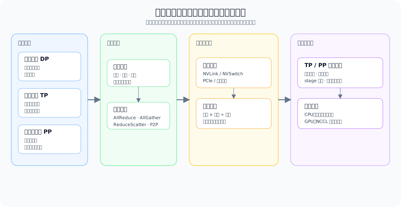
大模型训练从单卡扩展到多卡后，性能取决于两件事：每张卡如何切分数据、张量或网络层，以及切分后需要交换多少数据。先从 DP、TP、PP 的切分对象入手，再追踪 All-Reduce、All-Gather、Reduce-Scatter 和点到点传输，最后把链路带宽与同步等待放回吞吐判断。

本节沿着“并行方式 → 数据交换 → 拓扑带宽 → 计算与通信重叠”推进。完成后，你应能为一种并行方案指出主要通信原语，做出通信量级的初步估算，并解释链路带宽和同步等待如何影响并行收益。

关键词： DP, TP, PP

---

前置阅读

导语： 先复习 GPU 内存层级和设备间连接，再用 DP、TP、PP 的示例回答三个问题：数据放在哪里、哪些数据需要交换、链路带宽如何改变并行收益。

• 03. GPU Architecture and Memory | GPU 物理架构与内存层级
• Group 1C: Distributed Communication and Memory Sharing | 1C: 多卡通信与显存共享

---

Q1：DP、TP、PP 分别如何切分数据、张量和层？

点击展开查看解析

先分别看清数据并行（DP）、张量并行（TP）和流水线并行（PP）各自切分什么，再说明它们组合后为什么称为 3D 并行，最后追踪切分产生的数据交换。

• DP：不同卡处理不同数据批次，再同步梯度。
• TP：把单层中的大张量切到多卡上共同计算。
• PP：把不同层切到不同设备或设备组上形成流水线。

将 DP、TP、PP 组合使用时，通常称为 3D 并行。它们的目标不是“越多越好”，而是让模型、算力和通信拓扑能一起匹配。先把切分对象、主要交换的数据和常见通信方式分开看：

并行方式	切分对象	主要交换的数据	常见通信方式
DP	不同数据批次	梯度或参数更新结果	常见 All-Reduce
TP	层内张量或激活	局部激活、局部结果	可能使用 All-Gather、Reduce-Scatter 或 All-Reduce
PP	不同层或阶段	相邻阶段的激活	点到点传输，并伴随流水线等待

### Q1小验证：对照并行维度的切分对象与通信关注点

逐项检查每种并行方式切分什么、需要交换什么，以及对应的通信方式。

def three_d_parallel(dp, tp, pp):
    """组合 DP、TP、PP 三个并行维度，返回切分关系和通信关注点。"""
    if any(value <= 0 for value in (dp, tp, pp)):
        raise ValueError('dp、tp、pp 必须为正数')
    # 先记录三个并行维度，再观察它们组合后的 worker 数量和通信关系。
    return {
        'dp_groups': dp,
        'tp_shards': tp,
        'pp_stages': pp,
        'effective_workers': dp * tp * pp,
        'partition_axis': {'dp': 'data', 'tp': 'tensor', 'pp': 'layers'},
        'communication_focus': {
            'dp': 'gradient synchronization',
            'tp': 'activation gather / reduce-scatter',
            'pp': 'stage activation transfer',
        },
    }

cases = [
    three_d_parallel(8, 1, 1),
    three_d_parallel(4, 2, 2),
    three_d_parallel(2, 4, 4),
]
for case in cases:
    print(case)
assert cases[0]['partition_axis'] == {'dp': 'data', 'tp': 'tensor', 'pp': 'layers'}
assert 'gradient' in cases[1]['communication_focus']['dp']
assert 'activation' in cases[2]['communication_focus']['pp']
print('3D parallelism = DP × TP × PP')

Q2：All-Reduce、All-Gather、Reduce-Scatter 分别有什么区别？

点击展开查看解析

这三种集合通信原语的区别，先从每张卡的输入、输出和数据变化看起。下面的形状只是数据流示意；实际耗时还会受到消息大小、world size、拓扑、collective 算法和通信库实现影响。代码只模拟这些输入 / 输出形状，不执行真实 NCCL 通信。

通信原语	每卡输入	每卡输出	数据变化	常见使用场景
All-Reduce	局部张量	相同形状的归约结果	归约后复制到每卡	DP 梯度同步
All-Gather	局部分片	拼接后的完整张量	收集各卡分片	TP 激活或参数收集
Reduce-Scatter	较大的局部输入	归约后的局部结果	先归约，再切分	分片梯度或参数同步

### Q2小验证：通信原语如何改变每张卡看到的数据

先观察“聚合”“收集”“切分再发回”三种数据流。

def collective_shape(kind, world_size, local_shape):
    """返回集合通信的输入 / 输出形状；只模拟数据流，不执行真实通信。"""
    if world_size <= 0 or not local_shape or any(dim <= 0 for dim in local_shape):
        raise ValueError('world_size 和 local_shape 必须为正数')
    table = {
        'allreduce': {'operation': 'reduce + broadcast', 'input_per_rank': local_shape, 'output_per_rank': local_shape},
        'allgather': {'operation': 'gather all pieces', 'input_per_rank': local_shape, 'output_per_rank': (local_shape[0] * world_size, *local_shape[1:])},
        'reducescatter': {'operation': 'reduce then scatter', 'input_per_rank': (local_shape[0] * world_size, *local_shape[1:]), 'output_per_rank': local_shape},
    }
    if kind not in table:
        raise ValueError(f'未知通信原语: {kind}')
    return table[kind]

world_size = 4
local_shape = (8, 1024)
for kind in ['allreduce', 'allgather', 'reducescatter']:
    print(kind, '->', collective_shape(kind, world_size, local_shape))
assert collective_shape('allreduce', 4, (8, 1024))['output_per_rank'] == (8, 1024)
assert collective_shape('allgather', 4, (8, 1024))['output_per_rank'] == (32, 1024)
assert collective_shape('reducescatter', 4, (8, 1024))['input_per_rank'] == (32, 1024)
try:
    collective_shape('unknown', 4, (8, 1024))
except ValueError:
    print('✅ 非法通信原语校验通过')
else:
    raise AssertionError('未知通信原语应报错')

Q3：通信拓扑如何改变通信代价？

点击展开查看解析

先区分通信发生在哪里，再比较相同消息大小经过不同链路的理想传输时间。下表中的带宽统一按 Gb/s 表示，只是教学示例，不代表所有 GPU、主板、驱动或网络配置；真实实验应以 nvidia-smi topo -m、NCCL 测试或厂商规格为准。

通信位置	常见链路	教学示例带宽（Gb/s）	主要特点	适合承载的通信
GPU 机内	NVLink / NVSwitch	900 级	带宽高、延迟较低	高频 TP 或集合通信
GPU 到 CPU	PCIe	64 级	带宽较低、路径更长	参数搬运、低频同步
跨节点	网络互连	以实际集群为准	受网络和拓扑影响大	低频或可重叠通信

### Q3小验证：相同消息经过不同链路需要多久

在相同消息大小下，比较不同链路的理想传输时间。

def bandwidth_ratio(intra_gbps=900, inter_gbps=64):
    """返回同一单位下的链路带宽比；数值只是拓扑教学假设。"""
    if intra_gbps <= 0 or inter_gbps <= 0:
        raise ValueError('intra_gbps 和 inter_gbps 必须为正数')
    return intra_gbps / inter_gbps

print(f'ratio ≈ {bandwidth_ratio():.1f}x')

Q4：如何根据通信代价选择并行策略？

点击展开查看解析

用下面的条件表把并行方式、带宽、同步频率和计算重叠连接起来。表中的“初步策略”只表示通信账本给出的方向，不替代真实系统测量。

观察条件	可能的风险	初步策略
DP 需要跨低带宽链路同步梯度	梯度通信拖慢每轮更新	减少同步频率，或提高通信与计算重叠
TP 需要跨低带宽链路频繁同步	集合通信成为瓶颈	缩小 TP 范围，优先放在高速互连内
PP 跨阶段传输激活较多	阶段间等待、pipeline bubble	调整 stage 边界或 micro-batch
通信时间接近计算时间	扩展收益下降	尝试通信与计算重叠
只有理想带宽估算	无法确认真实部署收益	把同一 workload 带入后续系统实验

### Q4小验证：比较并行策略的通信占比

def comm_time_ms(size_mb, bandwidth_gbps, sync_rounds=1):
    """估算重复同步的理想单向传输时间；只作为带宽下界。"""
    if size_mb < 0:
        raise ValueError('size_mb must be non-negative')
    if bandwidth_gbps <= 0 or sync_rounds <= 0:
        raise ValueError('bandwidth_gbps 和 sync_rounds 必须为正数')
    # MB -> Mb，除以 Gb/s，再换算为毫秒；忽略协议、同步和重叠开销。
    return size_mb * 8 / bandwidth_gbps * sync_rounds

payload_mb = 256
sync_rounds = 4
nvlink_gbps = 900
pcie_gbps = 64
nvlink_time = comm_time_ms(payload_mb, nvlink_gbps, sync_rounds)
pcie_time = comm_time_ms(payload_mb, pcie_gbps, sync_rounds)
ratio = pcie_time / nvlink_time

print(f'{payload_mb} MB × {sync_rounds} sync rounds over NVLink: {nvlink_time:.2f} ms')
print(f'{payload_mb} MB × {sync_rounds} sync rounds over PCIe: {pcie_time:.2f} ms')
print(f'PCIe / NVLink time ratio: {ratio:.1f}x')

def parallel_strategy_report(strategy, payload_mb, bandwidth_gbps, sync_rounds, compute_ms):
    """用理想通信时间比较 DP、TP、PP 的通信占比；不模拟真实 collective。"""
    if strategy not in {'DP', 'TP', 'PP'}:
        raise ValueError('strategy 必须是 DP、TP 或 PP')
    if compute_ms <= 0:
        raise ValueError('compute_ms 必须为正数')
    communication_ms = comm_time_ms(payload_mb, bandwidth_gbps, sync_rounds)
    ratio = communication_ms / compute_ms
    if strategy == 'DP':
        action = '检查梯度同步频率与重叠'
    elif strategy == 'TP':
        action = '优先放在高速互连内'
    else:
        action = '检查 stage 边界与 micro-batch'
    return {
        'strategy': strategy,
        'communication_ms': round(communication_ms, 3),
        'communication_compute_ratio': round(ratio, 3),
        'next_action': action,
    }

reports = [
    parallel_strategy_report('DP', 256, 64, 4, 20),
    parallel_strategy_report('TP', 256, 900, 8, 20),
    parallel_strategy_report('PP', 64, 64, 2, 20),
]
print('并行策略通信占比：', reports)
assert {row['strategy'] for row in reports} == {'DP', 'TP', 'PP'}

---

相关阅读

本节可以继续接到 NCCL 原语、并行策略选择和通信调度；论文与开源实现用于补充真实系统中的数据交换路径。

• NCCL Documentation：查看 AllReduce、AllGather、ReduceScatter 和拓扑选择。
• Megatron-LM：观察张量并行、流水线并行和数据并行如何组合。
• Megatron-LM: Training Multi-Billion Parameter Language Models：理解大模型并行训练中的通信组织。
• 20. NCCL and AllReduce Basics | NCCL 与 AllReduce 基础
• 26. Parallel Strategy Decision Framework | 并行策略决策框架
• 27. Communication Scheduling Optimization | 通信调度优化

---