3. 正运动学与逆运动学实现

上一讲推导出了 FK 公式，这一讲把公式变成工程代码。

---

3.1 从公式到代码

上一讲我们用矩阵连乘推导出了 FK 公式：

x = L1 * cos(θ1) + L2 * cos(θ1 + θ2)
y = L1 * sin(θ1) + L2 * sin(θ1 + θ2)

这一讲的任务是：把公式变成工程代码。

"工程代码"和"能跑的代码"的区别在于：

能跑的代码	工程代码
只处理正常情况	处理边界情况和错误
结果对不对靠肉眼看	有自动验证机制
只有一个函数	有清晰的接口设计
没有注释	注释说明单位、假设、限制

这些习惯从现在开始养成，后面接入 ROS2 时会省很多麻烦。

---

3.2 IK 解析推导——余弦定理怎么用

3.2.1 问题转化

已知末端位置 (x, y)，求 θ1 和 θ2。

先看 θ2：末端到 base 原点的距离是固定的，记为 r：

r = sqrt(x² + y²)

现在看 base、关节 2、末端这三个点构成的三角形：

        末端 (x, y)
       ╱           ╲
  L2  ╱             ╲  r
     ╱               ╲
  关节2 ─────────────── base
           L1

三条边长度分别是：L1、L2、r。

这是一个已知三边求角的问题，用余弦定理：

c² = a² + b² - 2ab * cos(C)

把 r 当作 c，L1 当作 a，L2 当作 b，C 就是 θ2 的补角……

实际上更直接的推导是：把 FK 公式两边平方相加：

x² + y² = (L1*cos(θ1) + L2*cos(θ1+θ2))² + (L1*sin(θ1) + L2*sin(θ1+θ2))²

展开化简（利用 sin²+cos²=1）：

x² + y² = L1² + L2² + 2*L1*L2*cos(θ2)

因此：

cos(θ2) = (x² + y² - L1² - L2²) / (2 * L1 * L2)

---

3.3 双解的几何意义——肘上与肘下

3.3.1 为什么有两个解

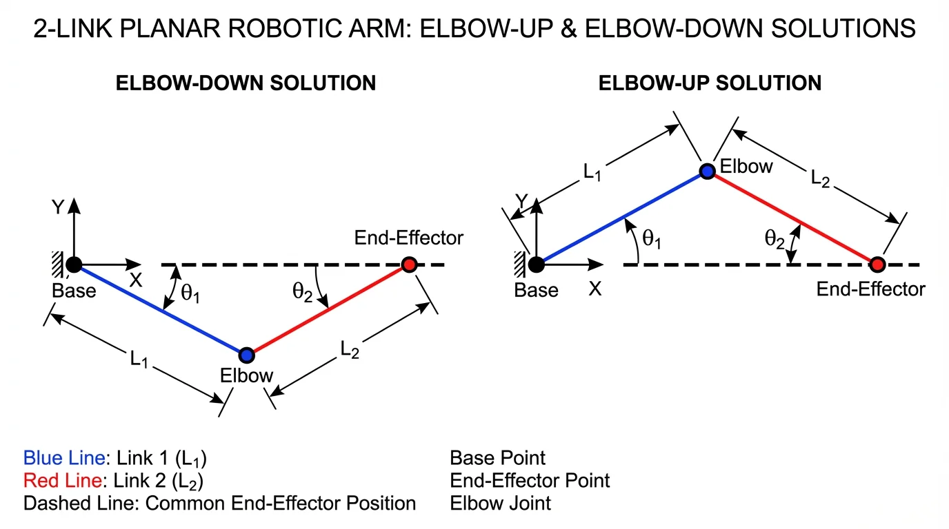
cos(θ2) = 0.7071 对应两个角度：

θ2 = +45°（肘下解，elbow down）
θ2 = -45°（肘上解，elbow up）

这两个解对应机械臂的两种不同构型，但末端位置完全相同：

肘下解（θ2 = +45°）        肘上解（θ2 = -45°）

y                           y
│     末端*                 │     末端*
│    ╱                      │    ╱
│   ╱ ← 关节2向下弯          │   ╱
│  *                        │  ╱
│ ╱                         │ * ← 关节2向上弯
│╱                          │╱
└──── x                     └──── x

两连杆平面机械臂：肘下解与肘上解对比

3.3.2 实际工程中怎么选

两个解都是数学上正确的，选哪个取决于：

• 避障：哪种构型不会碰到障碍物
• 关节限位：哪种构型的关节角在允许范围内
• 连续性：从当前构型出发，哪种解更近（避免突变）

在 MoveIt 2 里，IK 求解器会根据这些约束自动选择，但理解双解的存在是调试的基础。

3.3.3 什么情况只有一个解或无解

情况一：目标在工作空间边界（r = L1 + L2）
  两根连杆完全伸直，θ2 = 0°，只有一个解

情况二：目标太近（r = |L1 - L2|）
  两根连杆完全折叠，θ2 = ±180°，只有一个解

情况三：目标超出工作空间（r > L1 + L2 或 r < |L1 - L2|）
  cos(θ2) 超出 [-1, 1] 范围，无解

---

3.4 可达性判断——工作空间的几何直觉

3.4.1 工作空间是一个圆环

两连杆机械臂的工作空间（末端能到达的所有点）是一个圆环：

        最大可达距离 = L1 + L2
       ╭─────────────╮
      ╱               ╲
     │   ╭─────────╮   │
     │  ╱           ╲  │
     │ │  不可达区域  │ │  ← 最小可达距离 = |L1 - L2|
     │  ╲           ╱  │
     │   ╰─────────╯   │
      ╲               ╱
       ╰─────────────╯
              O (base)

类比：想象你手里拿着一根绳子（L1），绳子末端再绑一根绳子（L2）。你能触到的范围就是这个圆环。

3.4.2 可达性判断公式

r = sqrt(x² + y²)

可达条件：|L1 - L2| <= r <= L1 + L2

3.4.3 三个边界测试用例

给定 L1 = 1.0，L2 = 1.0：

import math

def check_reachability(x, y, L1, L2):
    r = math.sqrt(x**2 + y**2)
    r_max = L1 + L2
    r_min = abs(L1 - L2)
    if r > r_max:
        return False, f"太远：r={r:.3f} > 最大可达 {r_max:.3f}"
    if r < r_min:
        return False, f"太近：r={r:.3f} < 最小可达 {r_min:.3f}"
    return True, f"可达：r={r:.3f} 在 [{r_min:.3f}, {r_max:.3f}] 内"

L1, L2 = 1.0, 1.0
test_points = [(2.0, 0.0), (0.0, 0.0), (3.0, 0.0), (1.0, 1.0)]
for x, y in test_points:
    ok, msg = check_reachability(x, y, L1, L2)
    print(f"({x}, {y}): {'✓' if ok else '✗'} {msg}")

输出：

(2.0, 0.0): ✓ 可达：r=2.000 在 [0.000, 2.000] 内
(0.0, 0.0): ✗ 太近：r=0.000 < 最小可达 0.000
(3.0, 0.0): ✗ 太远：r=3.000 > 最大可达 2.000
(1.0, 1.0): ✓ 可达：r=1.414 在 [0.000, 2.000] 内

注意：当 L1 = L2 时，最小可达距离为 0，原点理论上可达（两杆完全折叠）。当 L1 ≠ L2 时，原点不可达。

---

3.5 完整 Python 实现（工程版）

# two_link_kinematics.py
# 运行方式：python3 two_link_kinematics.py

import math


def forward_kinematics(theta1_deg, theta2_deg, L1=1.0, L2=1.0):
    """
    两连杆平面机械臂正运动学

    参数：
        theta1_deg: 关节1角度（度），相对 base 坐标系
        theta2_deg: 关节2角度（度），相对连杆1坐标系
        L1: 连杆1长度（米），默认 1.0
        L2: 连杆2长度（米），默认 1.0

    返回：
        (x, y): 末端位置（米）
    """
    theta1 = math.radians(theta1_deg)
    theta2 = math.radians(theta2_deg)

    x = L1 * math.cos(theta1) + L2 * math.cos(theta1 + theta2)
    y = L1 * math.sin(theta1) + L2 * math.sin(theta1 + theta2)

    return x, y


def inverse_kinematics(x, y, L1=1.0, L2=1.0):
    """
    两连杆平面机械臂逆运动学

    参数：
        x, y: 目标末端位置（米）
        L1: 连杆1长度（米），默认 1.0
        L2: 连杆2长度（米），默认 1.0

    返回：
        dict，包含两组解：
        {
            "elbow_down": (theta1_deg, theta2_deg),  # 肘下解，theta2 > 0
            "elbow_up":   (theta1_deg, theta2_deg),  # 肘上解，theta2 < 0
        }
        如果目标不可达，抛出 ValueError

    注意：
        返回角度单位为度
    """
    r_sq = x**2 + y**2
    r = math.sqrt(r_sq)

    # 可达性检查
    r_max = L1 + L2
    r_min = abs(L1 - L2)
    if r > r_max:
        raise ValueError(
            f"目标点 ({x:.3f}, {y:.3f}) 超出工作空间："
            f"距离 {r:.3f} m > 最大可达 {r_max:.3f} m"
        )
    if r < r_min:
        raise ValueError(
            f"目标点 ({x:.3f}, {y:.3f}) 在死区内："
            f"距离 {r:.3f} m < 最小可达 {r_min:.3f} m"
        )

    # 用余弦定理求 θ2
    cos_theta2 = (r_sq - L1**2 - L2**2) / (2 * L1 * L2)
    # 防止浮点误差导致 acos 输入略微超出 [-1, 1]
    cos_theta2 = max(-1.0, min(1.0, cos_theta2))

    theta2_down = math.acos(cos_theta2)   # 肘下解：θ2 > 0
    theta2_up   = -theta2_down            # 肘上解：θ2 < 0

    def solve_theta1(theta2):
        # k1、k2 是辅助变量，来自对 FK 公式的变形：
        #   x = (L1 + L2*cos(θ2))*cos(θ1) - L2*sin(θ2)*sin(θ1)
        #   y = (L1 + L2*cos(θ2))*sin(θ1) + L2*sin(θ2)*cos(θ1)
        # 令 k1 = L1 + L2*cos(θ2)，k2 = L2*sin(θ2)，则：
        #   x = k1*cos(θ1) - k2*sin(θ1)
        #   y = k1*sin(θ1) + k2*cos(θ1)
        # 这是标准的 atan2 形式：θ1 = atan2(y,x) - atan2(k2,k1)
        k1 = L1 + L2 * math.cos(theta2)
        k2 = L2 * math.sin(theta2)
        return math.atan2(y, x) - math.atan2(k2, k1)

    theta1_down = solve_theta1(theta2_down)
    theta1_up   = solve_theta1(theta2_up)

    return {
        "elbow_down": (math.degrees(theta1_down), math.degrees(theta2_down)),
        "elbow_up":   (math.degrees(theta1_up),   math.degrees(theta2_up)),
    }

---

3.6 用 FK 验证 IK——round-trip 测试

3.6.1 为什么需要 round-trip 测试

IK 求出关节角之后，怎么知道结果是对的？

最直接的方法：把 IK 的结果代回 FK，看末端位置是否和目标一致。

目标点 (x, y)
    ↓ IK
关节角 (θ1, θ2)
    ↓ FK
末端位置 (x', y')
    ↓ 比较
误差 = sqrt((x-x')² + (y-y')²)

如果误差 < 1e-10，说明实现正确。

3.6.2 完整验证代码

import math


def verify_ik(x_target, y_target, L1=1.0, L2=1.0, tol=1e-10):
    """
    验证 IK 结果是否正确（round-trip 测试）

    参数：
        x_target, y_target: 目标末端位置
        L1, L2: 连杆长度
        tol: 允许的最大误差（米）

    返回：
        打印验证结果
    """
    print(f"\n目标点: ({x_target:.4f}, {y_target:.4f})")
    print("-" * 50)

    try:
        solutions = inverse_kinematics(x_target, y_target, L1, L2)
    except ValueError as e:
        print(f"IK 失败: {e}")
        return

    for name, (t1, t2) in solutions.items():
        x_fk, y_fk = forward_kinematics(t1, t2, L1, L2)
        error = math.sqrt((x_target - x_fk)**2 + (y_target - y_fk)**2)
        status = "✓" if error < tol else "✗"
        print(f"  {name:12s}: θ1={t1:7.2f}°, θ2={t2:7.2f}°  "
              f"→ FK=({x_fk:.4f}, {y_fk:.4f})  误差={error:.2e} {status}")


# 测试用例
L1, L2 = 1.0, 0.8

# 正常情况
verify_ik(1.0731, 1.2727, L1, L2)

# 边界情况：两杆完全伸直
verify_ik(1.8, 0.0, L1, L2)

# 边界情况：目标在 y 轴上
verify_ik(0.0, 1.5, L1, L2)

# 不可达情况
verify_ik(3.0, 0.0, L1, L2)

输出：

目标点: (1.0731, 1.2727)
--------------------------------------------------
  elbow_down  : θ1=  30.00°, θ2=  45.00°  → FK=(1.0731, 1.2727)  误差=2.22e-16 ✓
  elbow_up    : θ1=  75.00°, θ2= -45.00°  → FK=(1.0731, 1.2727)  误差=2.22e-16 ✓

目标点: (1.8000, 0.0000)
--------------------------------------------------
  elbow_down  : θ1=   0.00°, θ2=   0.00°  → FK=(1.8000, 0.0000)  误差=0.00e+00 ✓
  elbow_up    : θ1=   0.00°, θ2=  -0.00°  → FK=(1.8000, 0.0000)  误差=0.00e+00 ✓

目标点: (0.0000, 1.5000)
--------------------------------------------------
  elbow_down  : θ1=  56.79°, θ2=  56.41°  → FK=(0.0000, 1.5000)  误差=4.44e-16 ✓
  elbow_up    : θ1= 123.21°, θ2= -56.41°  → FK=(0.0000, 1.5000)  误差=4.44e-16 ✓

目标点: (3.0000, 0.0000)
--------------------------------------------------
IK 失败: 目标点 (3.000, 0.000) 超出工作空间：距离 3.000 m > 最大可达 1.800 m

误差在 1e-16 量级，是浮点数精度的极限，说明实现完全正确。

---

3.7 matplotlib 可视化

3.7.1 安装依赖

pip install matplotlib

3.7.2 画出机械臂两种构型

# visualize_arm.py
# 运行方式：python3 visualize_arm.py

import math
import matplotlib.pyplot as plt
import matplotlib.patches as patches


def plot_arm(ax, theta1_deg, theta2_deg, L1, L2, color, label):
    """在给定的坐标轴上画出机械臂"""
    theta1 = math.radians(theta1_deg)
    theta2 = math.radians(theta2_deg)

    # 三个关键点
    x0, y0 = 0, 0                                          # base
    x1 = L1 * math.cos(theta1)                            # 关节2
    y1 = L1 * math.sin(theta1)
    x2 = x1 + L2 * math.cos(theta1 + theta2)              # 末端
    y2 = y1 + L2 * math.sin(theta1 + theta2)

    # 画连杆
    ax.plot([x0, x1], [y0, y1], color=color, linewidth=3, label=label)
    ax.plot([x1, x2], [y1, y2], color=color, linewidth=3, linestyle='--')

    # 画关节
    ax.plot(x0, y0, 'ko', markersize=10)   # base
    ax.plot(x1, y1, 'o', color=color, markersize=8)   # 关节2
    ax.plot(x2, y2, '*', color=color, markersize=12)  # 末端

    # 标注末端坐标
    ax.annotate(f'({x2:.2f}, {y2:.2f})',
                xy=(x2, y2), xytext=(x2 + 0.05, y2 + 0.05),
                fontsize=9, color=color)


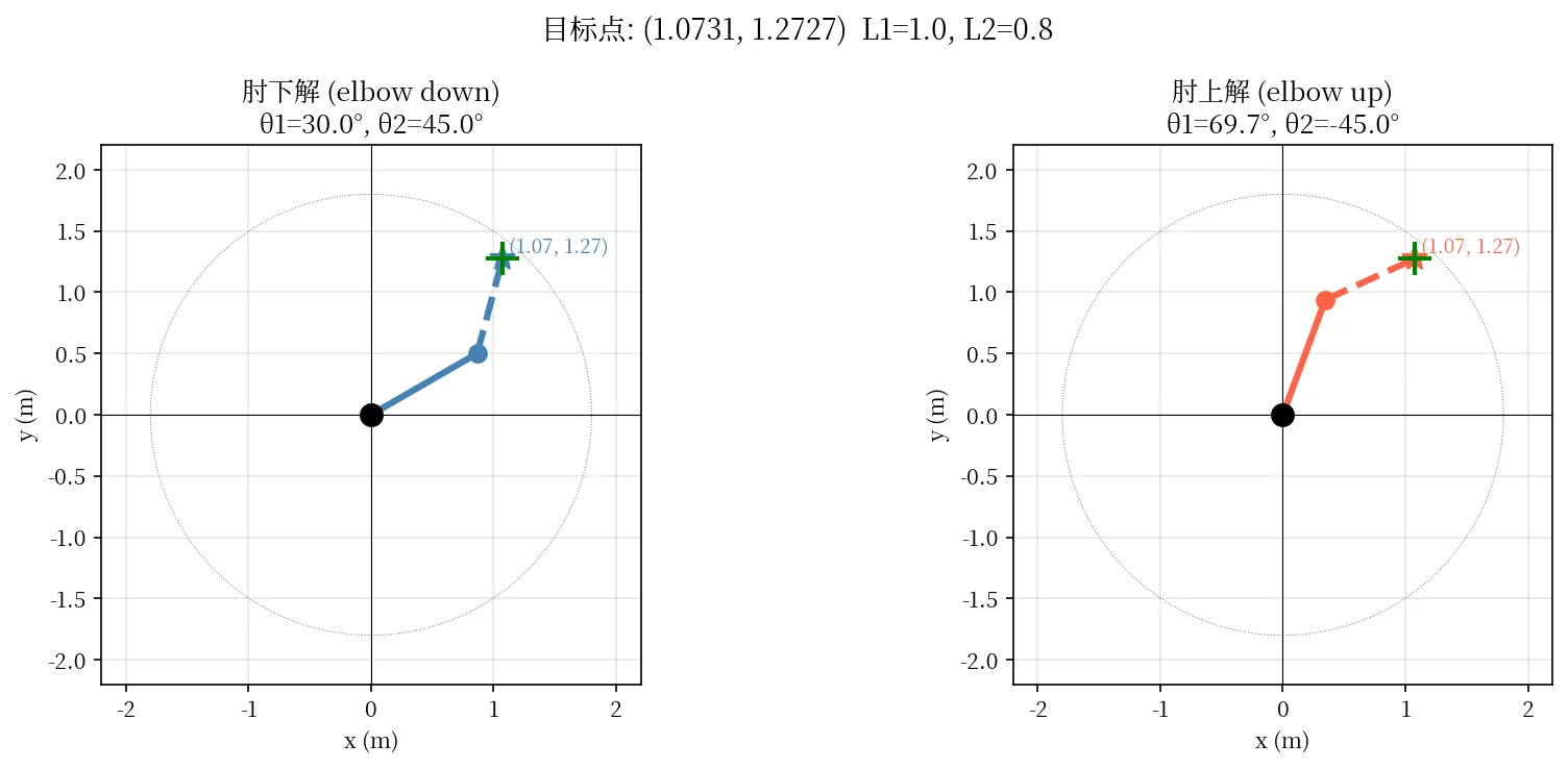
def visualize_solutions(x_target, y_target, L1=1.0, L2=0.8):
    """可视化 IK 的两种解"""
    solutions = inverse_kinematics(x_target, y_target, L1, L2)

    fig, axes = plt.subplots(1, 2, figsize=(12, 5))
    fig.suptitle(f'目标点: ({x_target}, {y_target})  L1={L1}, L2={L2}',
                 fontsize=13)

    colors = {'elbow_down': 'steelblue', 'elbow_up': 'tomato'}
    titles = {'elbow_down': '肘下解 (elbow down)', 'elbow_up': '肘上解 (elbow up)'}

    for ax, (name, (t1, t2)) in zip(axes, solutions.items()):
        plot_arm(ax, t1, t2, L1, L2, colors[name], name)

        # 画工作空间边界
        theta_range = [i * math.pi / 180 for i in range(361)]
        ax.plot([math.cos(t) * (L1 + L2) for t in theta_range],
                [math.sin(t) * (L1 + L2) for t in theta_range],
                'gray', linewidth=0.5, linestyle=':')

        # 标注目标点
        ax.plot(x_target, y_target, 'g+', markersize=15, markeredgewidth=2)

        ax.set_xlim(-2.2, 2.2)
        ax.set_ylim(-2.2, 2.2)
        ax.set_aspect('equal')
        ax.grid(True, alpha=0.3)
        ax.axhline(0, color='k', linewidth=0.5)
        ax.axvline(0, color='k', linewidth=0.5)
        ax.set_title(f'{titles[name]}\nθ1={t1:.1f}°, θ2={t2:.1f}°')
        ax.set_xlabel('x (m)')
        ax.set_ylabel('y (m)')

    plt.tight_layout()
    plt.savefig('arm_solutions.png', dpi=150, bbox_inches='tight')
    print("图片已保存为 arm_solutions.png")
    plt.show()


# 运行可视化
visualize_solutions(1.0731, 1.2727, L1=1.0, L2=0.8)

运行后会生成一张图，左边是肘下解，右边是肘上解，末端位置相同但构型不同。

matplotlib IK 可视化输出示例

---

3.8 常见错误

3.8.1 错误一：角度单位混用

# 错误：把度数直接传给 math.sin
x = L1 * math.cos(30) + L2 * math.cos(30 + 45)  # 30 被当成弧度！

# 正确：先换算成弧度
theta1 = math.radians(30)
theta2 = math.radians(45)
x = L1 * math.cos(theta1) + L2 * math.cos(theta1 + theta2)

怎么发现这个错误：结果数值看起来"差不多对"但不完全对，因为小角度时弧度和度数数值接近。用 round-trip 测试可以立刻发现。

---

3.8.2 错误二：acos 输入越界

# 错误：直接调用 acos，没有处理浮点误差
cos_theta2 = (r_sq - L1**2 - L2**2) / (2 * L1 * L2)
theta2 = math.acos(cos_theta2)  # 如果 cos_theta2 = 1.0000000000000002，会抛出异常

# 正确：先 clip 到 [-1, 1]
cos_theta2 = max(-1.0, min(1.0, cos_theta2))
theta2 = math.acos(cos_theta2)

什么时候会触发：目标点刚好在工作空间边界时，浮点运算可能产生极小的误差，导致 cos_theta2 略微超出 [-1, 1]。

---

3.8.3 错误三：只保留一组 IK 解

# 错误：只返回肘下解
theta2 = math.acos(cos_theta2)  # 只取正值

# 正确：同时返回两组解
theta2_down = math.acos(cos_theta2)
theta2_up   = -theta2_down

后果：在某些构型下，肘下解可能超出关节限位或碰到障碍物，但肘上解是可行的。只保留一组解会让规划器无法找到可行路径。

---

3.8.4 错误四：没有验证 IK 结果

写完 IK 函数后，一定要用 round-trip 测试验证。不验证的话，公式里一个符号写错（比如 + 写成 -），结果看起来"有数字"但完全错误。

---

本讲核心总结

概念	一句话理解
FK 公式来源	关节2位置 + 第二段连杆在全局方向的投影
IK 用余弦定理	把 FK 公式两边平方相加，消去 θ1，得到 cos(θ2)
双解	arccos 有正负两个值，对应肘上/肘下两种构型
工作空间	圆环，内径 |L1-L2|，外径 L1+L2
round-trip 测试	IK 结果代回 FK，误差应 < 1e-10
acos 越界	边界情况下浮点误差会导致输入略超 [-1,1]，必须 clip

---

参考代码

本讲对应的完整参考代码位于：

ros_ws/scripts/lesson_03_two_link_kinematics.py

文件内容：FK、IK 完整实现（含双解、可达性检查、round-trip 验证、matplotlib 可视化），含详细原理注释。

直接运行（无需 ROS2 环境）：

python3 $ROS_WS/scripts/lesson_03_two_link_kinematics.py

第4讲会把 forward_kinematics / inverse_kinematics 函数移入 ROS2 包 my_robot_basics，作为节点的算法核心复用。

---

下一讲预告

4. ROS2 工程基础

这一讲的 FK 和 IK 函数现在是独立的 Python 脚本，用 python3 two_link_kinematics.py 直接运行。下一讲我们会：

• 创建 ROS2 工作空间和第一个功能包 my_robot_basics
• 理解 package.xml、setup.py、colcon build 的作用
• 把 FK/IK 函数放进 ROS2 节点，用 ros2 run 启动
• 掌握 ros2 node list 等常用 CLI 工具

从这里开始，纯数学代码和 ROS2 工程正式接轨。