hello-rocm

第 2 章：解密 AI 加速器——从软件栈到硬件架构

实验环境
设备: AMD AI+ MAX395
GPU: Radeon 8060S
架构: gfx1151 (RDNA 3)
ROCm 版本: 7.x
系统: Ubuntu 24.04 / 22.04

本章学习目标

通过本章，你将理解三件核心事情：

软件调用链路：PyTorch 代码如何经过 HIP → HSA → Driver → GPU 执行
思维范式转变：从 CPU 的"低延迟"到 GPU 的"高吞吐"，SIMT 模型的工作原理
硬件架构原理：AMD GPU 的 CU、LDS、HBM，以及内存带宽的重要性

2.1 从 Python 到 GPU：一次代码执行的完整旅程

当你写下 x + y 这样的 PyTorch 代码时，你知道这行代码经历了多少层"翻译"才最终在 GPU 上执行吗？这一节，我们用 Linux 的工具来追踪整个调用链路。

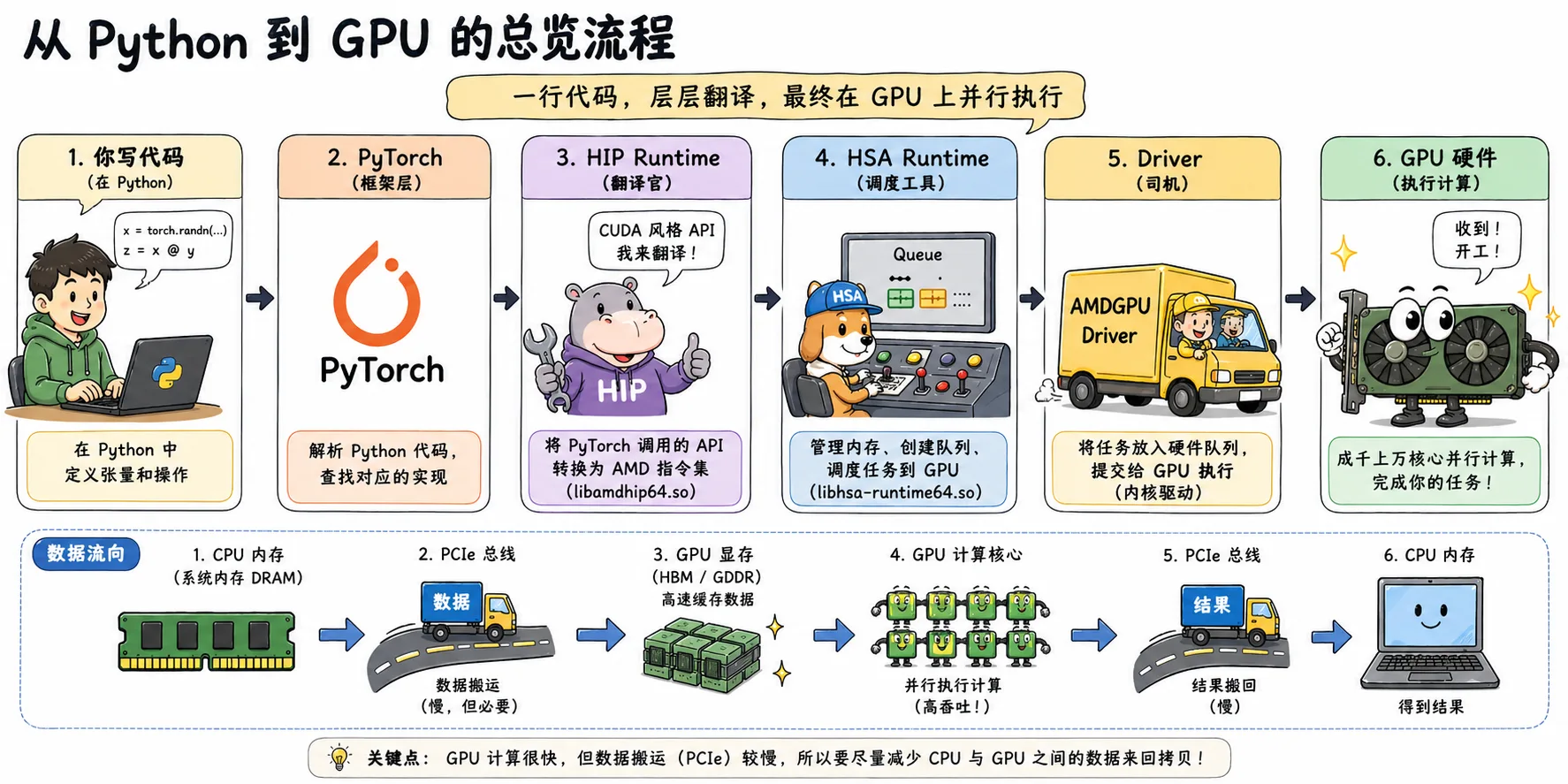
图2.1 从 Python 到 GPU 的总览流程：PyTorch 代码经过 HIP、HSA、Driver，最终在 GPU 上并行执行

2.1.1 黑盒解密：用 `ldd` 追踪 PyTorch 的依赖链路

PyTorch 只是一个高层封装，真正在 GPU 上干活的是底层的 ROCm 软件栈。让我们用 ldd 工具（查看动态库依赖）来揭开这个黑盒。

追踪命令

bash

# 找到 torch 库的路径
TORCH_LIB=$(python -c "import torch; print(torch.__file__)" | sed 's/__init__.py/lib/')

# 查看核心依赖 (过滤出 amd/rocm 相关的)
ldd $TORCH_LIB/libtorch_python.so | grep -E "amd|hip|hsa"

输出示例

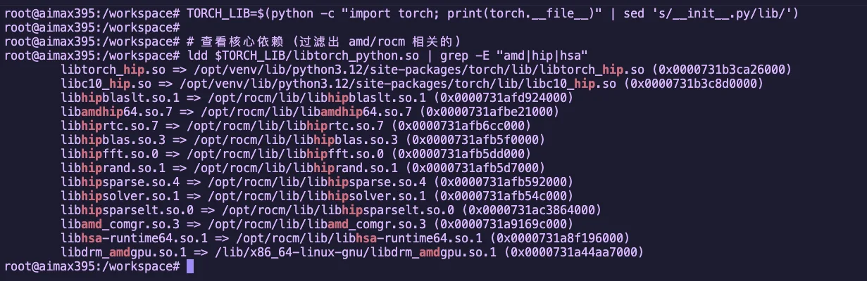
图2.2 ldd 查看 PyTorch 的 ROCm 依赖库

这些库构成了 ROCm 软件栈的核心，我们逐个拆解：

四大核心组件

组件	库名	职责	对应关系
翻译官	`libamdhip64.so`	将 CUDA 风格的 API 调用转换为 AMD 的指令	NVIDIA 的 `libcudart`
工头	`libhsa-runtime64.so`	真正调度 GPU、管理内存、让显卡开始干活	HSA 异构计算基础架构
技能包	`hipblas`/`hipfft` 等	高性能数学库（矩阵乘法、FFT 等）	NVIDIA 的 cuBLAS/cuFFT
编译器前端	`libamd_comgr.so`	动态编译 HIP 代码为二进制对象	NVIDIA 的 NVRTC

数学库详解

库名	作用	应用场景
`hipblas`	矩阵运算（BLAS）	线性层、矩阵乘法
`hipfft`	快速傅里叶变换	信号处理、某些注意力机制
`hiprand`	随机数生成	Dropout、噪声注入
`hipsparse`	稀疏矩阵运算	稀疏注意力机制

为什么需要这些数学库？
这些库是 AMD 工程师用汇编语言手写优化的，性能比你自己写的 HIP 代码快 10-100 倍。当你跑 Qwen 模型时，大量的矩阵运算就是由 hipblas 完成的。

2.1.2 全景图解：完整调用链路

前面的图用漫画方式展示了“一行 Python 代码如何一路跑到 GPU 上”。

现在我们换成更工程化的视角，把这条链路按软件栈分层拆开：

关键数据流

阶段	位置	任务
1. CPU 端	系统内存	准备数据、调用 API
2. PCIe 总线	总线传输	数据从系统内存搬运到显存
3. GPU 端	GPU 核心	Compute Units 并行执行计算
4. 返回	总线传输	结果从显存搬回系统内存

2.1.3 编译器视角：ROCm 如何用 LLVM/Clang 把高层代码"降维"

你写的 Python/HIP 代码，GPU 是看不懂的。编译器需要做一系列转换才能让 GPU 执行。

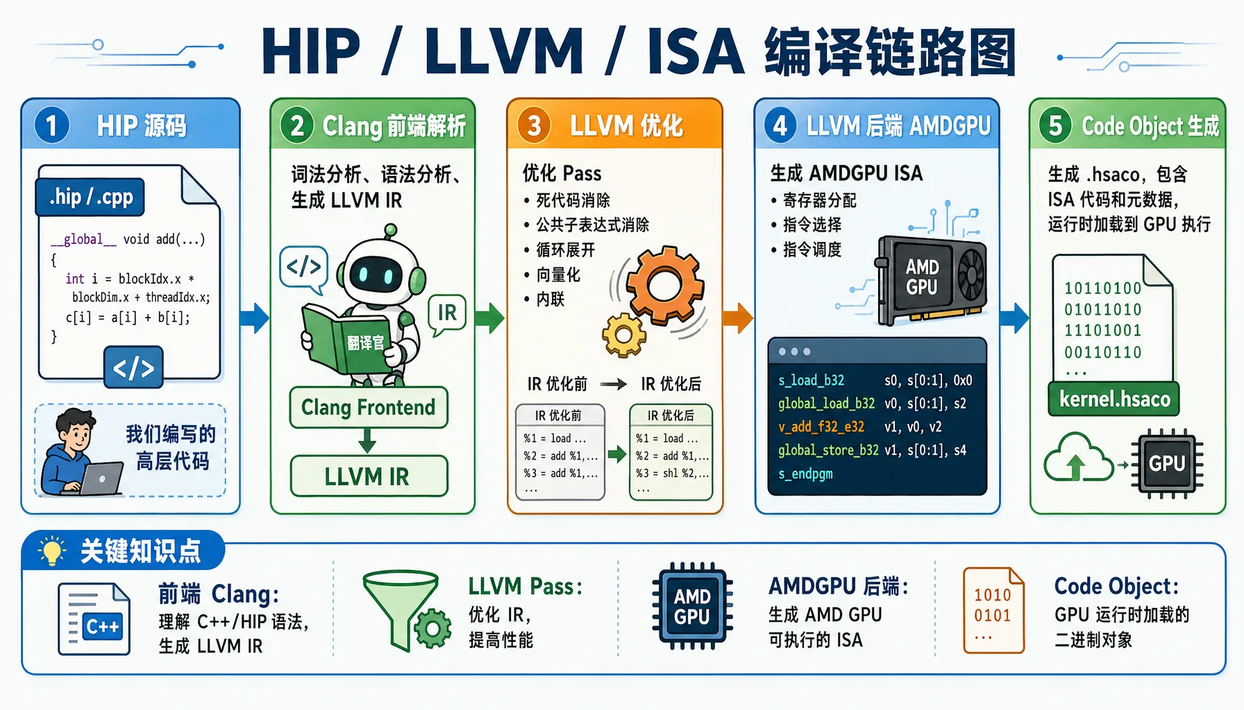
图2.3 HIP / LLVM / ISA 编译链路：从 C++/HIP 源码到 GPU 可执行二进制

示例：一个简单的 HIP 函数如何被编译

实战演练：让我们用实际的编译命令输出 LLVM IR 和 ISA。

创建文件 simple_add.cpp：

cpp

// file: src/infra/decode-ai-accelerator/code/simple_add.cpp
#include <hip/hip_runtime.h>
#include <iostream>

__global__ void add(float* a, float* b, float* c, int n) {
    int i = blockIdx.x * blockDim.x + threadIdx.x;
    if (i < n) {
        c[i] = a[i] + b[i];
    }
}

int main() {
    int n = 1024;
    size_t bytes = n * sizeof(float);

    float *a, *b, *c;
    hipMalloc(&a, bytes);
    hipMalloc(&b, bytes);
    hipMalloc(&c, bytes);

    float *h_a = new float[n];
    float *h_b = new float[n];
    for(int i = 0; i < n; i++) {
        h_a[i] = 1.0f;
        h_b[i] = 2.0f;
    }

    hipMemcpy(a, h_a, bytes, hipMemcpyHostToDevice);
    hipMemcpy(b, h_b, bytes, hipMemcpyHostToDevice);

    hipLaunchKernelGGL(add, dim3(1), dim3(n), 0, 0, a, b, c, n);
    hipDeviceSynchronize();

    float *h_c = new float[n];
    hipMemcpy(h_c, c, bytes, hipMemcpyDeviceToHost);

    std::cout << "Result: " << h_c[0] << ", " << h_c[n-1] << std::endl;

    delete[] h_a;
    delete[] h_b;
    delete[] h_c;
    hipFree(a);
    hipFree(b);
    hipFree(c);

    return 0;
}

方法 1：使用 hipcc 直接输出 LLVM IR

bash

# 输出未经优化的 LLVM IR
hipcc --offload-arch=gfx1151 \
      -emit-llvm \
      -S \
      -O0 \
      simple_add.cpp -o simple_add_O0.ll

# 输出优化后的 LLVM IR
hipcc --offload-arch=gfx1151 \
      -emit-llvm \
      -S \
      -O3 \
      simple_add.cpp -o simple_add_O3.ll

# 查看生成的 LLVM IR（只显示 GPU kernel 部分）
sed -n '/__CLANG_OFFLOAD_BUNDLE____START__ hip-amdgcn/,/__CLANG_OFFLOAD_BUNDLE____END__ hip-amdgcn/p' simple_add_O0.ll | grep -A 40 "define protected amdgpu_kernel"
sed -n '/__CLANG_OFFLOAD_BUNDLE____START__ hip-amdgcn/,/__CLANG_OFFLOAD_BUNDLE____END__ hip-amdgcn/p' simple_add_O3.ll | grep -A 40 "define protected amdgpu_kernel"

实际输出示例（未经优化的 LLVM IR -O0）：

llvm

; 生成的文件: simple_add_O0.ll
define protected amdgpu_kernel void @_Z3addPfS_S_i(ptr addrspace(1) noundef %0, ptr addrspace(1) noundef %1, ptr addrspace(1) noundef %2, i32 noundef %3) #4 {
  %5 = alloca i32, align 4, addrspace(5)
  %6 = alloca i32, align 4, addrspace(5)
  %7 = alloca i32, align 4, addrspace(5)
  %8 = alloca i32, align 4, addrspace(5)
  %9 = alloca i32, align 4, addrspace(5)
  %10 = alloca i32, align 4, addrspace(5)
  %11 = alloca ptr, align 8, addrspace(5)
  %12 = alloca ptr, align 8, addrspace(5)
  %13 = alloca ptr, align 8, addrspace(5)
  %14 = alloca ptr, align 8, addrspace(5)
  %15 = alloca ptr, align 8, addrspace(5)
  %16 = alloca ptr, align 8, addrspace(5)
  %17 = alloca i32, align 4, addrspace(5)
  %18 = alloca i32, align 4, addrspace(5)
  store ptr addrspace(1) %0, ptr addrspacecast(ptr addrspace(5) %11 to ptr), align 8
  %27 = load ptr, ptr addrspacecast(ptr addrspace(5) %11 to ptr), align 8
  store ptr addrspace(1) %1, ptr addrspacecast(ptr addrspace(5) %12 to ptr), align 8
  %28 = load ptr, ptr addrspacecast(ptr addrspace(5) %12 to ptr), align 8
  store ptr addrspace(1) %2, ptr addrspacecast(ptr addrspace(5) %13 to ptr), align 8
  %29 = load ptr, ptr addrspacecast(ptr addrspace(5) %13 to ptr), align 8
  %32 = call i64 @__ockl_get_group_id(i32 noundef 0) #17
  %33 = trunc i64 %32 to i32
  %36 = call i64 @__ockl_get_local_size(i32 noundef 0) #17
  %37 = trunc i64 %36 to i32
  %38 = mul i32 %33, %37
  %41 = call i64 @__ockl_get_local_id(i32 noundef 0) #17
  %42 = trunc i64 %41 to i32
  %43 = add i32 %38, %42
  store i32 %43, ptr addrspacecast(ptr addrspace(5) %18 to ptr), align 4
  %44 = load i32, ptr addrspacecast(ptr addrspace(5) %18 to ptr), align 4
  %45 = load i32, ptr addrspacecast(ptr addrspace(5) %17 to ptr), align 4
  %46 = icmp slt i32 %44, %45
  br i1 %46, label %47, label %63

47:
  %48 = load ptr, ptr addrspacecast(ptr addrspace(5) %14 to ptr), align 8
  %50 = sext i32 %49 to i64
  %52 = load float, ptr %51, align 4
  %58 = fadd contract float %52, %57
  store float %58, ptr %62, align 4
  br label %63

63:
  ret void
}
; O0 版本约 75 行代码

实际输出示例（优化后的 LLVM IR -O3）：

llvm

; 生成的文件: simple_add_O3.ll
define protected amdgpu_kernel void @_Z3addPfS_S_i(ptr addrspace(1) noundef readonly captures(none) %0, ...) local_unnamed_addr #0 {
  ; 无栈分配！所有变量都在寄存器中
  %5 = tail call i32 @llvm.amdgcn.workgroup.id.x()
  %6 = tail call ptr addrspace(4) @llvm.amdgcn.implicitarg.ptr()
  %8 = load i16, ptr addrspace(4) %7, align 4, !tbaa !6
  %9 = zext i16 %8 to i32
  %10 = mul i32 %5, %9
  %11 = tail call noundef range(i32 0, 1024) i32 @llvm.amdgcn.workitem.id.x()
  %12 = add i32 %10, %11
  %13 = icmp slt i32 %12, %3
  br i1 %13, label %14, label %22

14:
  %15 = sext i32 %12 to i64
  %19 = load float, ptr addrspace(1) %18, align 4, !tbaa !10
  %20 = load float, ptr addrspace(1) %17, align 4, !tbaa !10
  %21 = fadd contract float %19, %20
  store float %21, ptr addrspace(1) %16, align 4, !tbaa !10
  br label %22

22:
  ret void
}
; O3 版本仅约 35 行代码

O0 vs O3 关键差异对比
维度 O0 O3
栈使用 18 个 alloca（private memory）完全无栈分配
函数调用 @__ockl_get_group_id 等包装函数直接调用 @llvm.amdgcn.workgroup.id.x() intrinsic
代码量 约 75 行约 35 行（优化掉 50%）
内存访问 多次冗余 load/store 所有变量保持寄存器
TBAA 注解 无添加 !tbaa 用于类型别名分析优化
参数属性 无添加 readonly/captures(none) 帮助优化

维度	O0	O3
栈使用	18 个 alloca（private memory）	完全无栈分配
函数调用	`@__ockl_get_group_id` 等包装函数	直接调用 `@llvm.amdgcn.workgroup.id.x()` intrinsic
代码量	约 75 行	约 35 行（优化掉 50%）
内存访问	多次冗余 load/store	所有变量保持寄存器
TBAA 注解	无	添加 `!tbaa` 用于类型别名分析优化
参数属性	无	添加 `readonly`/`captures(none)` 帮助优化

（可选）输出 AMDGPU ISA 汇编代码：

bash

# 输出 ISA 汇编代码
hipcc --offload-arch=gfx1151 -S -O3 simple_add.cpp -o simple_add.s

# 查看生成的汇编（只显示 GPU kernel 部分）
sed -n '/__CLANG_OFFLOAD_BUNDLE____START__ hip-amdgcn/,/__CLANG_OFFLOAD_BUNDLE____END__ hip-amdgcn/p' simple_add.s | head -100

实际输出示例（AMDGPU ISA 汇编）：

asm

# __CLANG_OFFLOAD_BUNDLE____START__ hip-amdgcn-amd-amdhsa--gfx1151
        .amdgcn_target "amdgcn-amd-amdhsa--gfx1151"
        .amdhsa_code_object_version 6
        .text
        .protected      _Z3addPfS_S_i
        .globl  _Z3addPfS_S_i
        .p2align        8
        .type   _Z3addPfS_S_i,@function
_Z3addPfS_S_i:
; %bb.0:
        s_clause 0x1
        s_load_b32 s3, s[0:1], 0x2c
        s_load_b32 s4, s[0:1], 0x18
        s_waitcnt lgkmcnt(0)
        s_and_b32 s3, s3, 0xffff
        s_delay_alu instid0(SALU_CYCLE_1)
        v_mad_u64_u32 v[0:1], null, s2, s3, v[0:1]
        s_mov_b32 s2, exec_lo
        v_cmpx_gt_i32_e64 s4, v0
        s_cbranch_execz .LBB0_2
; %bb.1:
        s_load_b128 s[4:7], s[0:1], 0x0
        v_ashrrev_i32_e32 v1, 31, v0
        s_load_b64 s[0:1], s[0:1], 0x10
        s_delay_alu instid0(VALU_DEP_1) | instskip(SKIP_1) | instid1(VALU_DEP_1)
        v_lshlrev_b64 v[0:1], 2, v[0:1]
        s_waitcnt lgkmcnt(0)
        v_add_co_u32 v2, vcc_lo, s4, v0
        s_delay_alu instid0(VALU_DEP_1) | instskip(SKIP_1) | instid1(VALU_DEP_1)
        v_add_co_ci_u32_e64 v3, null, s5, v1, vcc_lo
        v_add_co_u32 v4, vcc_lo, s6, v0
        v_add_co_ci_u32_e64 v5, null, s7, v1, vcc_lo
        global_load_b32 v2, v[2:3], off
        global_load_b32 v3, v[4:5], off
        v_add_co_u32 v0, vcc_lo, s0, v0
        s_delay_alu instid0(VALU_DEP_1)
        v_add_co_ci_u32_e64 v1, null, s1, v1, vcc_lo
        s_waitcnt vmcnt(0)
        v_add_f32_e32 v2, v2, v3
        global_store_b32 v[0:1], v2, off
.LBB0_2:
        s_endpgm

关键汇编指令解读：

指令	说明
`s_load_b32`	标量加载：从常量内存加载到 SGPR
`v_mad_u64_u32`	向量乘加：计算线程全局 ID
`v_cmpx_gt_i32`	向量比较：边界检查，同时更新执行掩码
`global_load_b32`	全局内存加载：从显存读取数据
`v_add_f32_e32`	向量浮点加法：执行实际的加法运算
`global_store_b32`	全局内存存储：写回显存
`s_endpgm`	程序结束：终止 kernel 执行

为什么需要运行时编译（JIT）？

PyTorch 有一个强大的能力：运行时编译。当你写一个自定义算子时，PyTorch 会：

在运行时调用 hiprtc (HIP Runtime Compilation)
使用 libamd_comgr 编译你的 HIP 代码
生成适配当前 GPU 架构的二进制
加载到 GPU 执行

这就是为什么 PyTorch 能"动态编译" HIP 算子。

2.1.4 实战验证：手写第一个 HIP 程序

实战目标：现在我们跳过 Python，直接用 C++ 写一个 HIP 程序，验证整个调用链路。

创建文件 `hello_rocm.cpp`

cpp

// file: src/infra/decode-ai-accelerator/code/hello_rocm.cpp
#include <hip/hip_runtime.h>
#include <iostream>
#include <cstdlib>

#define HIP_CHECK(call)                                                         \
    do {                                                                        \
        hipError_t err = call;                                                  \
        if (err != hipSuccess) {                                                \
            std::cerr << "HIP Error: " << hipGetErrorString(err)                \
                      << " at line " << __LINE__ << std::endl;                  \
            std::exit(EXIT_FAILURE);                                            \
        }                                                                       \
    } while (0)

__global__ void vector_add(float *a, float *b, float *c, int n) {
    int i = blockDim.x * blockIdx.x + threadIdx.x;
    if (i < n) {
        c[i] = a[i] + b[i];
    }
}

int main() {
    int n = 1024;
    size_t bytes = n * sizeof(float);

    float *h_a, *h_b, *h_c;
    h_a = (float*)malloc(bytes);
    h_b = (float*)malloc(bytes);
    h_c = (float*)malloc(bytes);

    for(int i=0; i<n; i++) {
        h_a[i] = 1.0f;
        h_b[i] = 2.0f;
    }

    float *d_a, *d_b, *d_c;
    HIP_CHECK(hipMalloc(&d_a, bytes));
    HIP_CHECK(hipMalloc(&d_b, bytes));
    HIP_CHECK(hipMalloc(&d_c, bytes));

    HIP_CHECK(hipMemcpy(d_a, h_a, bytes, hipMemcpyHostToDevice));
    HIP_CHECK(hipMemcpy(d_b, h_b, bytes, hipMemcpyHostToDevice));

    hipLaunchKernelGGL(vector_add, dim3(1), dim3(n), 0, 0, d_a, d_b, d_c, n);
    HIP_CHECK(hipDeviceSynchronize());

    HIP_CHECK(hipMemcpy(h_c, d_c, bytes, hipMemcpyDeviceToHost));

    std::cout << "Element [0]: " << h_a[0] << " + " << h_b[0] << " = " << h_c[0] << std::endl;
    std::cout << "Element [1023]: " << h_a[1023] << " + " << h_b[1023] << " = " << h_c[1023] << std::endl;
    std::cout << ">>> ROCm HIP Kernel executed successfully on AMD GPU!" << std::endl;

    HIP_CHECK(hipFree(d_a)); HIP_CHECK(hipFree(d_b)); HIP_CHECK(hipFree(d_c));
    free(h_a); free(h_b); free(h_c);

    return 0;
}

编译并运行

bash

# 确认 hipcc 编译器是否就绪
which hipcc

# 编译
hipcc hello_rocm.cpp -o hello_rocm

# 运行
./hello_rocm

预期输出：

Element [0]: 1 + 2 = 3
Element [1023]: 1 + 2 = 3
>>> ROCm HIP Kernel executed successfully on AMD GPU!

图2.4 HIP 程序执行流程：CPU 负责调度，GPU 负责并行计算

程序执行流程

步骤	CPU 端	GPU 端
1. 分配内存	`malloc` 分配系统内存	`hipMalloc` 分配显存
2. 数据搬运	`hipMemcpy(H2D)` 把数据搬到显存	等待数据
3. 启动计算	`hipLaunchKernelGGL` 发射计算任务	1024 个线程并行计算
4. 同步	`hipDeviceSynchronize` 等待 GPU 完成	完成计算
5. 结果搬运	`hipMemcpy(D2H)` 把结果搬回内存	返回结果

恭喜！你刚刚完成了：第一次手动管理 GPU 内存、第一次手动启动 GPU 核函数、第一次完整走通了 PyTorch 底层的整个调用链路。

2.2 硬件思维革命：从 CPU 到 GPU 的范式转变

现在你已经知道代码如何跑到 GPU 上了，但一个更根本的问题是：为什么 AI 必须用 GPU？为什么 CPU 算不动？

答案在于 CPU 和 GPU 的设计哲学完全不同。

2.2.1 为什么 CPU 算不动 AI？

CPU 的设计哲学：低延迟

CPU 是为通用计算设计的，它的设计目标是：

设计目标	说明
低延迟	让单个任务尽可能快地完成
复杂控制流	支持复杂的分支预测、乱序执行
大缓存	L1/L2/L3 缓存减少内存访问延迟
少量强大的核心	通常 4-128 个核心，每个核心很强

CPU 擅长的任务：操作系统调度、数据库查询、逻辑复杂的业务代码、分支很多的算法。

AI 计算的特点：高吞吐

AI（深度学习）的负载完全不同：

计算特点	说明
数据并行	同时处理成千上万个数据
规则简单	主要是矩阵乘法、卷积
计算密集	每个数据需要大量浮点运算
内存带宽敏感	需要快速搬运大量数据

图2.5 CPU 低延迟 vs GPU 高吞吐设计哲学对比

CPU vs AI 需求的不匹配

CPU 的优化	AI 的需求	结果
大缓存减少延迟	需要高带宽搬数据	缓存太小，装不下模型
少量强大核心	需要数千弱核心并行	并行度不够
复杂分支预测	简单重复计算	分支预测器浪费资源

性能对比：ResNet-50 推理

我们用一个实际例子说明：在 CPU vs GPU 上运行 ResNet-50 推理。

实战演练：让我们在 Radeon 8060S (gfx1151) 上实际测试一下！

创建文件 bench_resnet.py：

python

# file: src/infra/decode-ai-accelerator/code/bench_resnet.py
import torch
import torchvision
import time

device_cpu = torch.device("cpu")
device_gpu = torch.device("cuda" if torch.cuda.is_available() else "cpu")

print(f"=== GPU 信息 ===")
if torch.cuda.is_available():
    print(f"GPU 设备: {torch.cuda.get_device_name(0)}")
    props = torch.cuda.get_device_properties(0)
    print(f"架构: {props.name}")
    print(f"显存: {props.total_memory / 1024**3:.1f} GB")
    print(f"计算能力: {props.major}.{props.minor}")
else:
    print("未检测到 GPU")

print("\n=== 加载 ResNet-50 模型 ===")
model = torchvision.models.resnet50(pretrained=True)
model.eval()

batch_size = 32
dummy_input = torch.randn(batch_size, 3, 224, 224)

# ========== CPU 推理测试 ==========
print("\n=== CPU 推理测试 ===")
model_cpu = model.to(device_cpu)

for _ in range(3):
    with torch.no_grad():
        _ = model_cpu(dummy_input)

start = time.time()
num_iterations = 10
with torch.no_grad():
    for _ in range(num_iterations):
        _ = model_cpu(dummy_input)
end = time.time()

cpu_time_ms = (end - start) / num_iterations * 1000 / batch_size
cpu_throughput = batch_size * num_iterations / (end - start)

print(f"CPU 平均延迟: {cpu_time_ms:.2f} ms/image")
print(f"CPU 吞吐量: {cpu_throughput:.2f} img/s")

# ========== GPU 推理测试 ==========
if torch.cuda.is_available():
    print("\n=== GPU 推理测试 ===")
    model_gpu = model.to(device_gpu)
    dummy_input_gpu = dummy_input.to(device_gpu)

    for _ in range(10):
        with torch.no_grad():
            _ = model_gpu(dummy_input_gpu)
        torch.cuda.synchronize()

    torch.cuda.synchronize()
    start = time.time()
    num_iterations = 100
    with torch.no_grad():
        for _ in range(num_iterations):
            _ = model_gpu(dummy_input_gpu)
    torch.cuda.synchronize()
    end = time.time()

    gpu_time_ms = (end - start) / num_iterations * 1000 / batch_size
    gpu_throughput = batch_size * num_iterations / (end - start)

    print(f"GPU 平均延迟: {gpu_time_ms:.2f} ms/image")
    print(f"GPU 吞吐量: {gpu_throughput:.2f} img/s")

    speedup = cpu_time_ms / gpu_time_ms
    print(f"\nGPU 加速比: {speedup:.1f}x")
    print(f"\n显存使用: {torch.cuda.max_memory_allocated() / 1024**3:.2f} GB")

运行测试：

bash

python bench_resnet.py

预期输出示例（在 Radeon 8060S 上）：

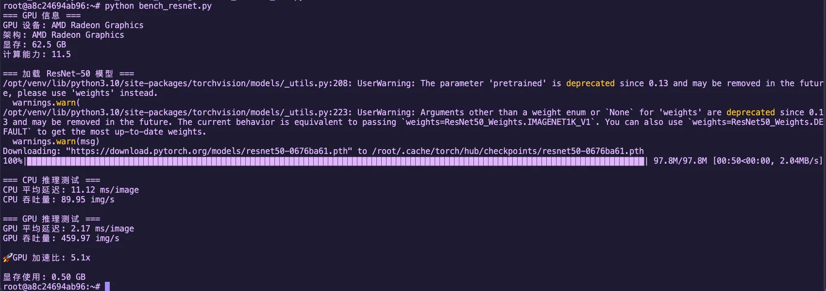
图2.7 ResNet-50 CPU vs GPU 推理性能对比（Radeon 8060S）

GPU vs CPU 性能对比分析
Radeon 8060S (gfx1151) 是消费级显卡，仍然有数十个 CU
每个 CU 能同时跑多个 wavefront（每个 wavefront 是 32/64 个线程）
对比 CPU：即使多核 CPU，并行度仍然远低于 GPU
差距的核心：GPU 用"人海战术"，CPU 是"精英战术"

2.2.2 SIMT 模型图解：单指令多线程的魔力

GPU 的核心技术是 SIMT (Single Instruction, Multiple Threads)，即"单指令多线程"。

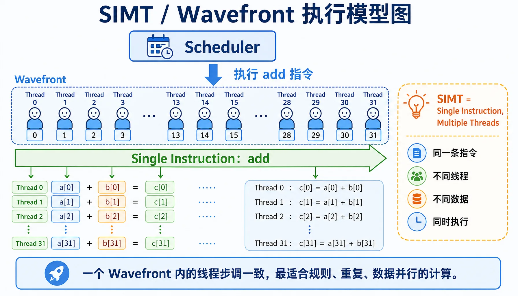
图2.8 SIMT / Wavefront 执行模型：同一条指令，多个线程处理不同数据

图2.9 控制单元 vs 运算单元：CPU 与 GPU 的晶体管分配差异

关键概念

概念	NVIDIA	AMD	说明
线程组	Warp (32线程)	Wavefront (32/64线程)	一组线程一起执行相同指令
分支发散	Warp Divergence	Wavefront Divergence	如果有 if-else 分支，性能会下降

上图说明了什么？
CPU：任务按顺序一个接一个执行，就像单人排队打饭
GPU：32个线程（一个 Wavefront）同时执行相同指令，就像一个班的同学一起做操

分支发散问题

当 wavefront 内的线程需要执行不同的代码路径时，就会发生分支发散，导致性能下降。

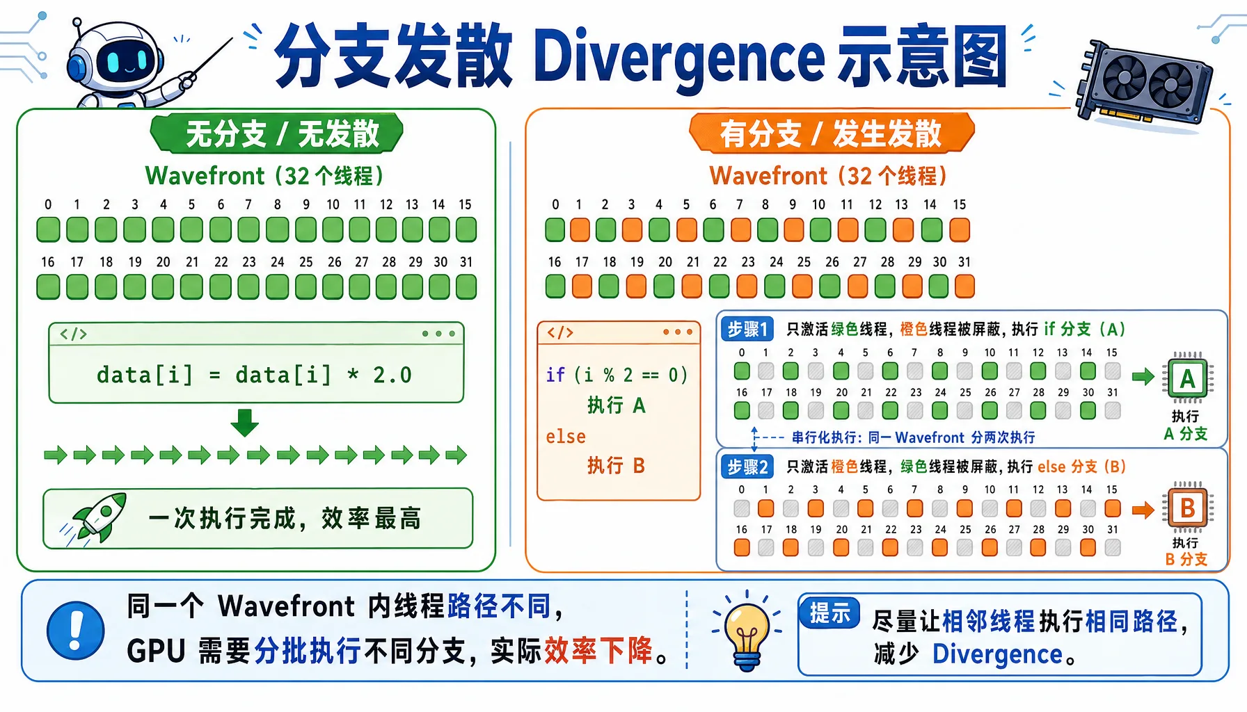
图2.10 分支发散：同一个 Wavefront 内线程走不同分支，会被拆成多次执行

糟糕的代码：

cpp

__global__ void bad_branch(float* data) {
    int i = threadIdx.x;
    if (i % 2 == 0) {  // 分支发散！
        data[i] *= 2.0f;
    } else {
        data[i] += 1.0f;
    }
}

执行情况：

Wavefront 包含线程 0-31
线程 0,2,4,... 执行 if 分支
线程 1,3,5,... 执行 else 分支
GPU 不得不串行执行两个分支，性能减半！

好的代码：

cpp

__global__ void good_branch(float* data) {
    int i = threadIdx.x;
    data[i] = data[i] * 2.0f + 1.0f;  // 无分支，全部并行
}

实战测试：分支发散性能影响

实战测试：让我们实际测试一下分支发散对性能的影响！

创建文件 bench_divergence.cpp：

cpp

// file: src/infra/decode-ai-accelerator/code/bench_divergence.cpp
#include <hip/hip_runtime.h>
#include <iostream>
#include <vector>
#include <cstdlib>

#define HIP_CHECK(call) \
    do { \
        hipError_t err = call; \
        if (err != hipSuccess) { \
            std::cerr << "HIP Error: " << hipGetErrorString(err) \
                      << " at line " << __LINE__ << std::endl; \
            std::exit(EXIT_FAILURE); \
        } \
    } while (0)

constexpr int WARP_SIZE = 32;

// 版本1：分支+同步的传统 reduction
__global__ void reduce_branchy(const float* __restrict__ in,
                               float* __restrict__ out,
                               int n) {
    extern __shared__ float sdata[];
    int tid = threadIdx.x;
    int global = blockIdx.x * blockDim.x * 2 + tid;

    float sum = 0.0f;
    if (global < n) sum += in[global];
    if (global + blockDim.x < n) sum += in[global + blockDim.x];
    sdata[tid] = sum;
    __syncthreads();

    for (int stride = blockDim.x / 2; stride > 0; stride >>= 1) {
        if (tid < stride) {
            sdata[tid] += sdata[tid + stride];
        }
        __syncthreads();
    }

    if (tid == 0) out[blockIdx.x] = sdata[0];
}

// wavefront shuffle sum
__device__ __forceinline__ float wf_reduce_sum(float v) {
    for (int offset = WARP_SIZE / 2; offset > 0; offset >>= 1) {
        v += __shfl_down(v, offset, WARP_SIZE);
    }
    return v;
}

__global__ void reduce_shuffle(const float* __restrict__ in,
                               float* __restrict__ out,
                               int n) {
    extern __shared__ float wf_sums[];

    int tid = threadIdx.x;
    int idx = blockIdx.x * blockDim.x * 2 + tid;

    float v = 0.0f;
    if (idx < n) v += in[idx];
    if (idx + blockDim.x < n) v += in[idx + blockDim.x];

    float wf_sum = wf_reduce_sum(v);

    int lane = tid % WARP_SIZE;
    int wid  = tid / WARP_SIZE;

    if (lane == 0) wf_sums[wid] = wf_sum;
    __syncthreads();

    if (wid == 0) {
        int num_waves = (blockDim.x + WARP_SIZE - 1) / WARP_SIZE;
        float x = (lane < num_waves) ? wf_sums[lane] : 0.0f;
        float block_sum = wf_reduce_sum(x);
        if (lane == 0) out[blockIdx.x] = block_sum;
    }
}

// Host：多轮 reduction 直到剩一个数
float run_reduce(const float* d_in, int n,
                 bool use_shuffle,
                 int threads, int iterations) {
    hipEvent_t start, stop;
    HIP_CHECK(hipEventCreate(&start));
    HIP_CHECK(hipEventCreate(&stop));

    int max_blocks = (n + (threads * 2 - 1)) / (threads * 2);
    float* d_buf1 = nullptr;
    float* d_buf2 = nullptr;
    HIP_CHECK(hipMalloc(&d_buf1, max_blocks * sizeof(float)));
    HIP_CHECK(hipMalloc(&d_buf2, max_blocks * sizeof(float)));

    auto launch_once = [&](int cur_n, const float* cur_in, float* cur_out) {
        int blocks = (cur_n + (threads * 2 - 1)) / (threads * 2);
        size_t smem = 0;
        if (use_shuffle) {
            int num_waves = (threads + WARP_SIZE - 1) / WARP_SIZE;
            smem = num_waves * sizeof(float);
            hipLaunchKernelGGL(reduce_shuffle, dim3(blocks), dim3(threads),
                               smem, 0, cur_in, cur_out, cur_n);
        } else {
            smem = threads * sizeof(float);
            hipLaunchKernelGGL(reduce_branchy, dim3(blocks), dim3(threads),
                               smem, 0, cur_in, cur_out, cur_n);
        }
        return blocks;
    };

    // warmup
    {
        int cur_n = n;
        const float* cur_in = d_in;
        float* cur_out = d_buf1;
        while (cur_n > 1) {
            int next_n = launch_once(cur_n, cur_in, cur_out);
            cur_n = next_n;
            cur_in = cur_out;
            cur_out = (cur_out == d_buf1) ? d_buf2 : d_buf1;
        }
        HIP_CHECK(hipDeviceSynchronize());
    }

    HIP_CHECK(hipEventRecord(start));
    for (int it = 0; it < iterations; ++it) {
        int cur_n = n;
        const float* cur_in = d_in;
        float* cur_out = d_buf1;

        while (cur_n > 1) {
            int next_n = launch_once(cur_n, cur_in, cur_out);
            cur_n = next_n;
            cur_in = cur_out;
            cur_out = (cur_out == d_buf1) ? d_buf2 : d_buf1;
        }
    }
    HIP_CHECK(hipEventRecord(stop));
    HIP_CHECK(hipEventSynchronize(stop));

    float ms = 0.0f;
    HIP_CHECK(hipEventElapsedTime(&ms, start, stop));

    HIP_CHECK(hipFree(d_buf1));
    HIP_CHECK(hipFree(d_buf2));
    HIP_CHECK(hipEventDestroy(start));
    HIP_CHECK(hipEventDestroy(stop));
    return ms;
}

int main() {
    int n = 1024 * 1024 * 1000; // 10M
    size_t bytes = n * sizeof(float);

    std::cout << "=== 向量求和（reduction）发散对比 ===\n";
    std::cout << "数据量: " << n << " (" << bytes / 1024.0 / 1024.0 << " MB)\n";
    std::cout << "WARP_SIZE(AMD wavefront): " << WARP_SIZE << "\n";

    std::vector<float> h(n, 1.0f);
    float* d_in = nullptr;
    HIP_CHECK(hipMalloc(&d_in, bytes));
    HIP_CHECK(hipMemcpy(d_in, h.data(), bytes, hipMemcpyHostToDevice));

    int threads = 256;
    int iterations = 50;

    std::cout << "\n=== reduce_branchy（分支+同步）===\n";
    float t1 = run_reduce(d_in, n, false, threads, iterations);
    std::cout << "总时间: " << t1 << " ms\n";
    std::cout << "平均每次: " << t1 / iterations << " ms\n";

    std::cout << "\n=== reduce_shuffle（shuffle 更少分支）===\n";
    float t2 = run_reduce(d_in, n, true, threads, iterations);
    std::cout << "总时间: " << t2 << " ms\n";
    std::cout << "平均每次: " << t2 / iterations << " ms\n";

    std::cout << "\n=== 对比 ===\n";
    float speedup = t1 / t2;
    std::cout << "shuffle 版本加速比: " << speedup << "x\n";
    std::cout << "性能提升: " << (speedup - 1.f) * 100.f << "%\n";

    HIP_CHECK(hipFree(d_in));
    return 0;
}

1
2
3
4
5
6
7
8
9
10
11
12
13
14
15
16
17
18
19
20
21
22
23
24
25
26
27
28
29
30
31
32
33
34
35
36
37
38
39
40
41
42
43
44
45
46
47
48
49
50
51
52
53
54
55
56
57
58
59
60
61
62
63
64
65
66
67
68
69
70
71
72
73
74
75
76
77
78
79
80
81
82
83
84
85
86
87
88
89
90
91
92
93
94
95
96
97
98
99
100
101
102
103
104
105
106
107
108
109
110
111
112
113
114
115
116
117
118
119
120
121
122
123
124
125
126
127
128
129
130
131
132
133
134
135
136
137
138
139
140
141
142
143
144
145
146
147
148
149
150
151
152
153
154
155
156
157
158
159
160
161
162
163
164
165
166
167
168
169
170
171
172
173
174
175
176
177
178
179
180
181
182

编译并运行：

bash

hipcc bench_divergence.cpp -o bench_divergence -O3
./bench_divergence

预期输出（在 Radeon 8060S 上）：

=== 向量求和（reduction）发散对比 ===
数据量: 1048576000 (4000 MB)
WARP_SIZE(AMD wavefront): 32

=== reduce_branchy（分支+同步）===
总时间: 1104.58 ms
平均每次: 22.0915 ms

=== reduce_shuffle（shuffle 更少分支）===
总时间: 960.202 ms
平均每次: 19.204 ms

=== 对比 ===
shuffle 版本加速比: 1.15036x
性能提升: 15.0359%

结论
从测试结果可以看到，使用 shuffle 指令减少分支发散带来了**约15%**的性能提升。虽然这个例子中提升不算巨大，但在某些场景下分支发散的影响会更大。在实际编写 GPU 代码时，应尽量避免在 wavefront 内部使用 if-else 分支。

为什么 32 或 64 个线程一组？

选项	优点	缺点
太少（如 8 个）	灵活	硬件调度开销大
太多（如 1024 个）	吞吐高	分支发散影响太大
32/64 个	刚好平衡并行度和灵活性

架构差异：老架构用 64，新架构（如 gfx1151）用 32

2.2.3 数据并行思维：如何把问题拆解成 GPU 能吃的形式

并行度分析：什么任务适合 GPU？

特征	适合 GPU	不适合 GPU
数据量	大数据集（>1000 元素）	小数据（<100 元素）
数据依赖	数据之间独立	数据之间有复杂依赖
计算模式	规则重复（矩阵、卷积）	复杂逻辑（递归、回溯）
分支	很少 if-else	很多 if-else
内存访问	连续访问	随机跳转

示例对比

适合 GPU：矩阵乘法（每个元素独立计算）、图像卷积（每个像素独立处理）、向量加法 c[i] = a[i] + b[i]

不适合 GPU：斐波那契数列（有依赖）、快速排序（分支太多）、图遍历（内存访问不规则）

内存访问模式：合并访问 vs 随机访问

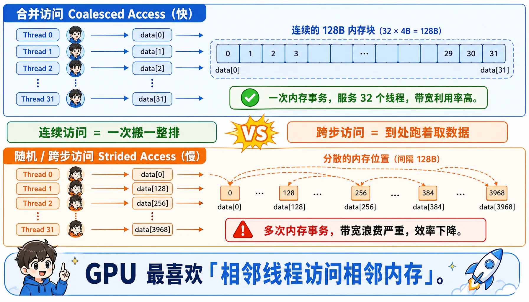
图2.11 合并访问 vs 随机访问：连续线程访问连续地址，访存效率最高

合并访问（Coalesced Access）- 快：

cpp

__global__ void good_access(float* data) {
    int i = threadIdx.x;  // 0, 1, 2, 3, ...
    // 连续的线程访问连续的内存 -> 一次内存事务
    float x = data[i];
}

线程0 -> data[0]  (字节 0-3)
线程1 -> data[1]  (字节 4-7)
线程2 -> data[2]  (字节 8-11)
...
线程31 -> data[31] (字节 124-127)
总共需要一次内存事务，一次读 128 字节，服务 32 个线程

随机访问（Strided Access）- 慢：

cpp

__global__ void bad_access(float* data) {
    int i = threadIdx.x;
    float x = data[i * 128];  // 跨度128
}

线程0 -> data[0]    -> 需要 1 次 128 字节事务
线程1 -> data[128]  -> 需要 1 次 128 字节事务
...
线程31 -> data[3968] -> 需要 1 次 128 字节事务
总共：32 次内存事务！

2.3 走进 AMD GPU 内部：硬件架构详解

现在我们深入 AMD GPU 的硬件，了解它的"内脏"是如何组织的。

2.3.1 Compute Unit (CU)：GPU 的"干活小组"

图2.12 AMD GPU Compute Unit 内部结构：SIMD、VGPR、SGPR、LDS 与调度器协同工作

CU 内部结构

一个 Compute Unit (CU) 是 GPU 的基本计算单元，它包含以下组件：

以 Radeon 8060S (gfx1151 架构) 为例

组件详情表：

组件	全称	功能比喻	关键特性
SIMD Units	单指令多数据单元	搬砖工：大家听同一个口令，搬不同的砖	每个 CU 通常有 4 个 SIMD，负责执行向量指令
VGPR	向量通用寄存器	工人的背包：每个线程私有的存储空间	极快但极贵。数量限制了能同时开工的工人数
SGPR	标量通用寄存器	队长的记事本：存储所有线程共用的数据	由标量单元处理，不占用向量单元资源
LDS	Local Data Store	队内的小仓库：同一个 CU 内的线程可以交换数据	速度比显存快 10-20 倍，用于 Block 内通讯

架构差异小贴士
CDNA (如 MI300)：专为计算设计，通常采用 Wave64 模式（64个线程一组）
RDNA (如 Radeon 7900)：专为游戏设计，通常采用 Wave32 模式（32个线程一组），但在计算任务中也可以编译为 Wave64

关键参数

参数	说明
CU 数量	Radeon 8060S 有数十个 CU（具体数量取决于芯片型号）
每个 CU 的 SIMD 数量	2-4 个
每个 CU 的 ALU 总数	数百个
理论峰值 FP32 吞吐	数 TFLOPS 级别

一个 CU 能同时跑多少线程？

这是 GPU 性能优化的关键问题。我们需要理解几个概念：

概念	说明
Work-Item（线程）	最小的执行单位
Work-Group（线程块）	一组线程，可以共享 LDS
Wavefront（波前）	32/64 个线程（取决于架构），一起执行相同指令

并发计算：

每个 wavefront 需要：32 或 64 个 VGPR（假设每个线程用 1 个寄存器）、一定数量的 LDS（如果使用）、指令槽位
每个 CU 可以同时跑 多个 wavefront（具体数量取决于架构）

CU 数量 x wavefront/CU x 32/64 thread/wavefront = 数万到数十万个线程

为什么线程束要超过物理核心数？

GPU 的物理 ALU 数量有限
但能跑远超物理核心数的线程（数倍到十倍！）
原因：内存延迟隐藏
- 当 Wave A 等待内存（需要 500 个周期）时，调度器瞬间切换到 Wave B 执行计算
- 只要排队的 Wave 足够多，CU 就永远不会停下来

Occupancy：资源利用率

图2.13 Occupancy 与寄存器压力：每个线程用的寄存器越多，同时驻留的 Wavefront 越少

公式：Occupancy = 实际并发 wavefront 数 / 理论最大 wavefront 数

影响因素：

资源	限制因素	优化方法
VGPR	每个线程用太多寄存器	减少寄存器使用
LDS	Work-group 用太多 LDS	减小 LDS 使用
指令槽位	Code 太大	减小代码大小

示例对比：

cpp

// 寄存器使用多 -> Occupancy 低
__global__ void heavy_register(float* data) {
    float a, b, c, d, e, f, g, h;  // 8个寄存器
    // ... 复杂计算
}

// 寄存器使用少 -> Occupancy 高
__global__ void light_register(float* data) {
    float a = data[threadIdx.x];
    a *= 2.0f;
    data[threadIdx.x] = a;
}

实战分析：使用 rocprof 工具分析 GPU 程序的 Occupancy 和性能指标

安装 rocprof（如果尚未安装）：

bash

# Ubuntu/Debian
sudo apt install hip-dev rocprofiler-dev roctracer-dev -y

# 验证安装
/opt/rocm/bin/rocprof --version

创建测试程序 test_occupancy.cpp：

cpp

// file: src/infra/decode-ai-accelerator/code/test_occupancy.cpp
#include <hip/hip_runtime.h>
#include <iostream>
#include <cstdlib>
#include <cmath>

#define HIP_CHECK(call) \
    do { \
        hipError_t err = call; \
        if (err != hipSuccess) { \
            std::cerr << "HIP Error: " << hipGetErrorString(err) \
                      << " at line " << __LINE__ << std::endl; \
            std::exit(EXIT_FAILURE); \
        } \
    } while (0)

// Heavy kernel: 让每个线程占用 >64 个 VGPR
__global__ void heavy_kernel(float* data, int n) {
    int idx = blockIdx.x * blockDim.x + threadIdx.x;
    if (idx < n) {
        volatile float v0 = data[idx];
        volatile float v1 = v0 * 1.01f;
        volatile float v2 = v1 * 1.02f;
        volatile float v3 = v2 * 1.03f;
        volatile float v4 = v3 * 1.04f;
        volatile float v5 = v4 * 1.05f;
        volatile float v6 = v5 * 1.06f;
        volatile float v7 = v6 * 1.07f;
        volatile float v8 = v7 * 1.08f;
        volatile float v9 = v8 * 1.09f;

        volatile float a[20];
        #pragma unroll
        for(int i=0; i<20; i++) {
            a[i] = v0 * (float)(i+1);
        }

        float sum = 0.0f;
        #pragma unroll
        for(int i=0; i<20; i++) {
            sum += a[i] * v1;
            sum -= v2 * v3;
            sum += v4 / (v5 + 1e-6f);
            sum *= (v6 + v7);
        }

        data[idx] = sum + v8 + v9;
    }
}

// 对照组：低寄存器占用 Kernel
__global__ void light_kernel(float* data, int n) {
    int idx = blockIdx.x * blockDim.x + threadIdx.x;
    if (idx < n) {
        float val = data[idx];
        val *= 2.0f;
        data[idx] = val;
    }
}

int main() {
    int n = 1024 * 1024 * 20; // 20M floats
    size_t bytes = n * sizeof(float);

    float *d_data;
    HIP_CHECK(hipMalloc(&d_data, bytes));

    const int threads = 256;
    const int blocks = (n + threads - 1) / threads;

    std::cout << "Data size: " << n << " elements (" << bytes/1024/1024 << " MB)" << std::endl;

    hipLaunchKernelGGL(light_kernel, dim3(blocks), dim3(threads), 0, 0, d_data, n);
    HIP_CHECK(hipDeviceSynchronize());

    std::cout << "=== Running heavy_kernel (High Register Pressure) ===" << std::endl;
    for(int i=0; i<5; i++) {
        hipLaunchKernelGGL(heavy_kernel, dim3(blocks), dim3(threads), 0, 0, d_data, n);
    }
    HIP_CHECK(hipDeviceSynchronize());

    std::cout << "\n=== Running light_kernel (Low Register Pressure) ===" << std::endl;
    for(int i=0; i<5; i++) {
        hipLaunchKernelGGL(light_kernel, dim3(blocks), dim3(threads), 0, 0, d_data, n);
    }
    HIP_CHECK(hipDeviceSynchronize());

    HIP_CHECK(hipFree(d_data));
    return 0;
}

编译并使用 rocprof 分析：

bash

# 编译
hipcc test_occupancy.cpp -o test_occupancy -O3

# 运行分析（会生成 results.csv）
rocprof --stats ./test_occupancy

# 查看生成的 CSV 文件
cat results.csv

rocprof 输出示例（节选关键字段）：

"Index","KernelName","arch_vgpr","scr","DurationNs"
0,"light_kernel(float*, int)",8,0,804159
1,"heavy_kernel(float*, int)",72,144,34497058

关键指标解读：

指标	Light Kernel	Heavy Kernel	差异倍数
arch_vgpr (向量寄存器)	8	72	9倍差距！
DurationNs (执行时间)	~720,000 ns (0.72ms)	~34,500,000 ns (34.5ms)	~48倍差距！
scr (Scratch Memory)	0	144	发生寄存器溢出 (Spill)

计算理论 Occupancy：

对于 gfx1151 架构（Radeon 8060S），每个 CU 的 VGPR 总数为 1024，每个 CU 的 LDS 总数为 64 KB，每个 CU 最大 wavefront 数为 32（理论值）。

python

# file: src/infra/decode-ai-accelerator/code/calc_occupancy.py

def calculate_occupancy_arch1151(vgpr_per_thread, lds_per_workgroup, threads_per_wg):
    total_physical_vgprs = 65536 // 4  # 16384
    wave_size = 32  # RDNA3 默认为 Wave32
    max_waves_per_simd = 32
    vgpr_granularity = 8

    aligned_vgpr = ((vgpr_per_thread + vgpr_granularity - 1) // vgpr_granularity) * vgpr_granularity
    vgpr_per_wave = aligned_vgpr * wave_size

    if vgpr_per_wave == 0:
        waves_by_vgpr = max_waves_per_simd
    else:
        waves_by_vgpr = total_physical_vgprs // vgpr_per_wave

    max_lds_bytes = 65536
    waves_per_wg = (threads_per_wg + wave_size - 1) // wave_size

    if lds_per_workgroup > 0:
        max_wgs_by_lds = max_lds_bytes // lds_per_workgroup
        waves_by_lds = max_wgs_by_lds * waves_per_wg
    else:
        waves_by_lds = max_waves_per_simd

    limit_waves = min(waves_by_vgpr, waves_by_lds, max_waves_per_simd)
    active_waves = (limit_waves // waves_per_wg) * waves_per_wg
    occupancy_pct = (active_waves / max_waves_per_simd) * 100

    return active_waves, occupancy_pct

print("=== 理论 Occupancy 计算 (RDNA3 / gfx1151) ===\n")

vgpr_heavy = 72
occ_heavy, pct_heavy = calculate_occupancy_arch1151(vgpr_heavy, 0, 256)
print(f"Heavy Kernel (VGPR={vgpr_heavy}):")
print(f"  Active Waves: {occ_heavy} / 32")
print(f"  Occupancy:    {pct_heavy:.1f}%")

vgpr_light = 8
occ_light, pct_light = calculate_occupancy_arch1151(vgpr_light, 0, 256)
print(f"\nLight Kernel (VGPR={vgpr_light}):")
print(f"  Active Waves: {occ_light} / 32")
print(f"  Occupancy:    {pct_light:.1f}%")

输出：

Heavy Kernel (VGPR=72):
  Active Waves: 8 / 32
  Occupancy:    12.5%

Light Kernel (VGPR=8):
  Active Waves: 32 / 32
  Occupancy:    100.0%

终极性能分析报告

性能杀手	现象	解释
1. 极低的并行度	Occupancy: 12.5%	CU 里有 87.5% 的计算资源是闲置的。原本可以跑 32 个 Wave，现在只能跑 8 个。GPU 无法通过切换线程来掩盖内存延迟，只能干等
2. 资源碎片化	Waves: 8 / 14	虽然 VGPR 够放 14 个 Wave，但因为 Workgroup 强制要求 8 个 Wave 一组，剩下的空位塞不下第二个 Workgroup，白白浪费了
3. 内存溢出 (最致命)	scr: 144 bytes	即使只有 12.5% 的 Occupancy，寄存器还是不够用！编译器被迫把部分变量"溢出"到慢速的 Scratch Memory 中，读写速度从几 TB/s 降到几百 GB/s

rocprof 常用命令
命令用途
rocprof --stats ./your_program 基础性能分析
rocprof --sys-trace --hip-trace ./your_program 追踪 HIP API 和 HSA 运行时
rocprof-plot -i results.csv -o report.html 生成 HTML 报告

命令	用途
`rocprof --stats ./your_program`	基础性能分析
`rocprof --sys-trace --hip-trace ./your_program`	追踪 HIP API 和 HSA 运行时
`rocprof-plot -i results.csv -o report.html`	生成 HTML 报告

优化建议
Occupancy > 70%：通常足够，不必追求 100%
减少寄存器使用：简化计算、复用变量
减小 LDS 使用：合理设计 workgroup 大小
使用 --maxrregcount=N 编译选项限制寄存器数

2.3.2 显存 (VRAM) vs 内存 (DRAM)：数据搬运的"过路费"

GPU 的另一个瓶颈是内存带宽。

HBM 带宽为什么这么贵？

内存类型	带宽	延迟	容量	价格
DDR4 (CPU)	~25 GB/s	~80 ns	128 GB	便宜
GDDR6 (游戏显卡)	~500 GB/s	~100 ns	24 GB	中等
HBM3 (MI300X)	5.3 TB/s	~120 ns	192 GB	非常贵

MI300X 的 5.3 TB/s 是什么概念？

相当于每秒搬运 1000 部高清电影
或者每秒搬运 整个维基百科（英文版）100 次

为什么 HBM 这么快？

技术	说明
堆叠封装	内存芯片直接堆在 GPU 旁边
超宽总线	4096 bit（对比 DDR4 的 64 bit）
短距离	信号传输路径只有几毫米

PCIe Gen5 的瓶颈

GPU 和 CPU 之间的数据搬运通过 PCIe 总线，它的速度远慢于 HBM：

PCIe 版本	带宽 (x16)	单向搬运 32 GB 时间
PCIe 4.0	32 GB/s	1 秒
PCIe 5.0	64 GB/s	0.5 秒

实际影响：

python

# 在 CPU 准备数据
x = torch.randn(1024, 1024, 1024)  # 4 GB

# 搬到 GPU
x = x.cuda()  # PCIe 5.0 需要 0.06 秒

# 在 GPU 计算
y = x @ x.T  # GPU 只需要几毫秒！

实战测试：让我们实际测试一下 PCIe 和 GPU 显存的带宽差异！

创建文件 bench_bandwidth.py：

python

# file: src/infra/decode-ai-accelerator/code/bench_bandwidth.py
import torch
import time

torch.manual_seed(42)

print("=== 内存带宽测试 ===")

if not torch.cuda.is_available():
    print("错误: 未检测到 GPU 设备！")
    exit(1)

device_id = 0
device = torch.device(f"cuda:{device_id}")
props = torch.cuda.get_device_properties(device_id)

print(f"GPU 设备: {torch.cuda.get_device_name(device_id)}")
print(f"架构: {props.name}")
print(f"总显存: {props.total_memory / 1024**3:.2f} GB\n")

# 测试 1: PCIe / 总线带宽 (CPU -> GPU)
print("=== 测试 1: PCIe 带宽 (CPU -> GPU) ===")

sizes_mb = [1, 10, 100, 500, 1024, 2048]

for size_mb in sizes_mb:
    size_bytes = size_mb * 1024 * 1024
    data_cpu = torch.randn(size_bytes // 4, dtype=torch.float32).pin_memory()

    data_cpu.to(device, non_blocking=True)
    torch.cuda.synchronize()

    start_event = torch.cuda.Event(enable_timing=True)
    end_event = torch.cuda.Event(enable_timing=True)

    start_event.record()
    data_gpu = data_cpu.to(device, non_blocking=True)
    end_event.record()

    torch.cuda.synchronize()
    elapsed_ms = start_event.elapsed_time(end_event)

    bandwidth_gbs = (size_mb / 1024) / (elapsed_ms / 1000)
    print(f"数据大小: {size_mb:4d} MB | 时间: {elapsed_ms:8.2f} ms | 带宽: {bandwidth_gbs:6.2f} GB/s")

# 测试 2: GPU 显存带宽 (GPU 内部)
print("\n=== 测试 2: GPU 显存带宽 (GPU 内部) ===")

test_sizes_mb = [100, 500, 1024]
max_safe_mb = int((props.total_memory / 1024**3) * 1024 * 0.4)
test_sizes_mb = [s for s in test_sizes_mb if s <= max_safe_mb]
if not test_sizes_mb: test_sizes_mb = [max_safe_mb]

for size_mb in test_sizes_mb:
    size_elements = (size_mb * 1024 * 1024) // 4
    src = torch.randn(size_elements, device=device, dtype=torch.float32)
    dst = torch.empty_like(src)

    dst.copy_(src)
    torch.cuda.synchronize()

    iterations = 50
    start_event = torch.cuda.Event(enable_timing=True)
    end_event = torch.cuda.Event(enable_timing=True)

    start_event.record()
    for _ in range(iterations):
        dst.copy_(src)
    end_event.record()

    torch.cuda.synchronize()
    total_time_ms = start_event.elapsed_time(end_event)
    avg_time_ms = total_time_ms / iterations

    total_data_gb = (size_mb * 2) / 1024
    bandwidth_gbs = total_data_gb / (avg_time_ms / 1000)

    print(f"数据大小: {size_mb:4d} MB | 时间: {avg_time_ms:8.2f} ms | 带宽: {bandwidth_gbs:6.2f} GB/s")

# 测试 3: 计算 vs 搬运
print("\n=== 测试 3: 计算时间 vs 数据搬运时间 ===")

data_size_mb = 256
N = 1024 * 1024 * (data_size_mb // 4)
data_cpu = torch.randn(N, dtype=torch.float32).pin_memory()

data_gpu = data_cpu.to(device, non_blocking=True)
torch.cuda.synchronize()

start_event = torch.cuda.Event(enable_timing=True)
end_event = torch.cuda.Event(enable_timing=True)

start_event.record()
data_gpu = data_cpu.to(device, non_blocking=True)
end_event.record()
torch.cuda.synchronize()
transfer_time_ms = start_event.elapsed_time(end_event)

torch.relu(data_gpu)
torch.cuda.synchronize()

start_event.record()
result = torch.relu(data_gpu)
end_event.record()
torch.cuda.synchronize()
compute_time_ms = start_event.elapsed_time(end_event)

print(f"数据搬运 (PCIe): {transfer_time_ms:.2f} ms")
print(f"简单计算 (GPU):  {compute_time_ms:.2f} ms (ReLU)")

ratio = transfer_time_ms / compute_time_ms
print(f"\n数据搬运比计算慢 {ratio:.1f} 倍！")
print("   (这证明了：频繁搬运数据会成为系统瓶颈)")

print("\n=== 理论带宽对比 ===")
print(f"PCIe 4.0 x16 理论带宽: 32 GB/s")
print(f"PCIe 5.0 x16 理论带宽: 64 GB/s")
print(f"LPDDR5X 理论带宽:    ~270 GB/s (Radeon 8060S)")

del data_cpu, data_gpu, src, dst, result
torch.cuda.empty_cache()

运行测试：

bash

python bench_bandwidth.py

输出（在 Radeon 8060S 上）：

=== 内存带宽测试 ===
GPU 设备: AMD Radeon 8060S
架构: AMD Radeon 8060S
总显存: 62.47 GB

=== 测试 1: PCIe 带宽 (CPU -> GPU) ===
数据大小:    1 MB | 时间:     0.29 ms | 带宽:   3.34 GB/s
数据大小:   10 MB | 时间:     0.29 ms | 带宽:  34.23 GB/s
数据大小:  100 MB | 时间:     1.22 ms | 带宽:  80.34 GB/s
数据大小:  500 MB | 时间:     6.11 ms | 带宽:  79.98 GB/s
数据大小: 1024 MB | 时间:    12.17 ms | 带宽:  82.19 GB/s
数据大小: 2048 MB | 时间:    24.79 ms | 带宽:  80.68 GB/s

=== 测试 2: GPU 显存带宽 (GPU 内部) ===
数据大小:  100 MB | 时间:     0.97 ms | 带宽: 201.87 GB/s
数据大小:  500 MB | 时间:     4.93 ms | 带宽: 197.89 GB/s
数据大小: 1024 MB | 时间:    10.19 ms | 带宽: 196.21 GB/s

=== 测试 3: 计算时间 vs 数据搬运时间 ===
数据搬运 (PCIe): 3.21 ms
简单计算 (GPU):  2.43 ms (ReLU)

数据搬运比计算慢 1.3 倍！
   (这证明了：频繁搬运数据会成为系统瓶颈)

关键发现 (Strix Halo 特有)
Host-to-Device 带宽惊人: ~80 GB/s（远超 PCIe 4.0/5.0，得益于 APU 统一内存架构）
GPU 显存带宽: ~200 GB/s（符合 LPDDR5X 四通道理论值）
数据搬运依然是瓶颈: 尽管拥有极高的互联带宽，数据传输耗时仍比 GPU 内部访存/计算慢 30% 以上
因此，即使在高性能 APU 上，减少 CPU-GPU 数据传输依然是优化的黄金法则。

解决方案：

方案	说明
数据预取	提前把数据搬到 GPU
流水线重叠	计算和数据搬运同时进行
模型并行	把模型分布到多个 GPU，减少跨卡通信

数据局部性优化：如何减少 GPU 饿肚子

GPU 计算快，但需要持续的数据流。如果数据供应不上，GPU 就会"饿肚子"。

饥饿示例：

cpp

__global__ void starving(float* data) {
    int i = threadIdx.x;
    // 每次访问都去显存拿 -> 高延迟
    for (int j = 0; j < 100; j++) {
        data[i] += data[i + j * 1024];
    }
}

优化：使用共享内存缓存

当你需要重复访问同一块数据时，LDS 是神器。

cpp

__global__ void optimized(float* data) {
    __shared__ float s_data[256];  // 片上共享内存
    int i = threadIdx.x;

    // 只访问一次显存，放到共享内存
    s_data[i] = data[i];
    __syncthreads();  // 等所有线程都加载完

    // 后续都从共享内存读（快10倍）
    for (int j = 0; j < 100; j++) {
        s_data[i] += s_data[(i + j) % 256];
    }

    data[i] = s_data[i];  // 最后写回
}

访问速度对比
存储层次延迟
显存 (HBM) 100-200 周期（慢）
共享内存 (LDS) 10-20 周期（快 10 倍）
寄存器 (VGPR) 1 周期（极快）

存储层次	延迟
显存 (HBM)	100-200 周期（慢）
共享内存 (LDS)	10-20 周期（快 10 倍）
寄存器 (VGPR)	1 周期（极快）

性能提升：通常能快 2-10 倍。

本章代码

本章涉及的完整源码位于 src/infra/decode-ai-accelerator/code/ 目录：

文件	说明
`hello_rocm.cpp`	第一个 HIP 程序：向量加法验证
`simple_add.cpp`	HIP 编译链路演示：LLVM IR / ISA 输出
`bench_resnet.py`	ResNet-50 CPU vs GPU 推理性能对比
`bench_divergence.cpp`	分支发散性能影响测试（reduction 对比）
`bench_bandwidth.py`	PCIe vs GPU 显存带宽测试
`calc_occupancy.py`	理论 Occupancy 计算脚本

本章小结

本章我们完成了以下内容：

用 ldd 追踪了 PyTorch → HIP → HSA → 驱动 → GPU 的完整调用链路。
理解了 CPU「低延迟」与 GPU「高吞吐」的设计哲学差异，以及 SIMT 执行模型。
深入 AMD GPU 硬件架构，掌握了 CU、VGPR、LDS、显存带宽等核心概念。
通过 rocprof 实测了 Occupancy、分支发散、内存带宽等关键性能指标。

实战练习

通过本章学习，你已经获得了多个完整的测试程序。现在请动手实践：

必做练习

追踪依赖

bash

TORCH_LIB=$(python -c "import torch; print(torch.__file__)" | sed 's/__init__.py/lib/')
ldd $TORCH_LIB/libtorch_python.so | grep -E "amd|hip|hsa"

手写 HIP：运行 hello_rocm.cpp，验证 GPU 能正常工作；尝试修改核函数实现向量乘法而非加法
性能对比测试

bash

python bench_resnet.py

分支发散测试

bash

hipcc bench_divergence.cpp -o bench_divergence -O3
./bench_divergence

内存带宽测试

bash

python bench_bandwidth.py

进阶练习

Occupancy 分析

bash

hipcc test_occupancy.cpp -o test_occupancy -O3
rocprof --stats ./test_occupancy
cat results.csv

优化挑战：尝试优化 bench_divergence.cpp 中的代码消除分支发散；尝试优化 test_occupancy.cpp 中的寄存器使用提高 Occupancy

第 2 章：解密 AI 加速器——从软件栈到硬件架构 ​

本章学习目标 ​

2.1 从 Python 到 GPU：一次代码执行的完整旅程 ​

2.1.1 黑盒解密：用 ldd 追踪 PyTorch 的依赖链路 ​

追踪命令 ​

输出示例 ​

四大核心组件 ​

数学库详解 ​

2.1.2 全景图解：完整调用链路 ​

关键数据流 ​

2.1.3 编译器视角：ROCm 如何用 LLVM/Clang 把高层代码"降维" ​

示例：一个简单的 HIP 函数如何被编译 ​

为什么需要运行时编译（JIT）？ ​

2.1.4 实战验证：手写第一个 HIP 程序 ​

创建文件 hello_rocm.cpp ​

编译并运行 ​

程序执行流程 ​

2.2 硬件思维革命：从 CPU 到 GPU 的范式转变 ​

2.2.1 为什么 CPU 算不动 AI？ ​

CPU 的设计哲学：低延迟 ​

AI 计算的特点：高吞吐 ​

CPU vs AI 需求的不匹配 ​

性能对比：ResNet-50 推理 ​

2.2.2 SIMT 模型图解：单指令多线程的魔力 ​

关键概念 ​

分支发散问题 ​

实战测试：分支发散性能影响 ​

为什么 32 或 64 个线程一组？ ​

2.2.3 数据并行思维：如何把问题拆解成 GPU 能吃的形式 ​

并行度分析：什么任务适合 GPU？ ​

示例对比 ​

内存访问模式：合并访问 vs 随机访问 ​

2.3 走进 AMD GPU 内部：硬件架构详解 ​

2.3.1 Compute Unit (CU)：GPU 的"干活小组" ​

CU 内部结构 ​

关键参数 ​

一个 CU 能同时跑多少线程？ ​

为什么线程束要超过物理核心数？ ​

Occupancy：资源利用率 ​

2.3.2 显存 (VRAM) vs 内存 (DRAM)：数据搬运的"过路费" ​

HBM 带宽为什么这么贵？ ​

MI300X 的 5.3 TB/s 是什么概念？ ​

为什么 HBM 这么快？ ​

PCIe Gen5 的瓶颈 ​

数据局部性优化：如何减少 GPU 饿肚子 ​

本章代码 ​

本章小结 ​

实战练习 ​

必做练习 ​

进阶练习 ​

参考资源 ​

第 2 章：解密 AI 加速器——从软件栈到硬件架构

本章学习目标

2.1 从 Python 到 GPU：一次代码执行的完整旅程

2.1.1 黑盒解密：用 `ldd` 追踪 PyTorch 的依赖链路

追踪命令

输出示例

四大核心组件

数学库详解

2.1.2 全景图解：完整调用链路

关键数据流

2.1.3 编译器视角：ROCm 如何用 LLVM/Clang 把高层代码"降维"

示例：一个简单的 HIP 函数如何被编译

为什么需要运行时编译（JIT）？

2.1.4 实战验证：手写第一个 HIP 程序

创建文件 `hello_rocm.cpp`

编译并运行

程序执行流程

2.2 硬件思维革命：从 CPU 到 GPU 的范式转变

2.2.1 为什么 CPU 算不动 AI？

CPU 的设计哲学：低延迟

AI 计算的特点：高吞吐

CPU vs AI 需求的不匹配

性能对比：ResNet-50 推理

2.2.2 SIMT 模型图解：单指令多线程的魔力

关键概念

分支发散问题

实战测试：分支发散性能影响

为什么 32 或 64 个线程一组？

2.2.3 数据并行思维：如何把问题拆解成 GPU 能吃的形式

并行度分析：什么任务适合 GPU？

示例对比

内存访问模式：合并访问 vs 随机访问

2.3 走进 AMD GPU 内部：硬件架构详解

2.3.1 Compute Unit (CU)：GPU 的"干活小组"

CU 内部结构

关键参数

一个 CU 能同时跑多少线程？

为什么线程束要超过物理核心数？

Occupancy：资源利用率

2.3.2 显存 (VRAM) vs 内存 (DRAM)：数据搬运的"过路费"

HBM 带宽为什么这么贵？

MI300X 的 5.3 TB/s 是什么概念？

为什么 HBM 这么快？

PCIe Gen5 的瓶颈

数据局部性优化：如何减少 GPU 饿肚子

本章代码

本章小结

实战练习

必做练习

进阶练习

参考资源