L11 · Domain Randomization

Course status: gpu-verified. The bilingual diagnostic paths, the complete CPU+EGL path, and the complete bounded-DR recording, readback, and provenance path on a reference R9700 have passed. The normal experiment needs camera rendering and remains GPU-recommended. The non-rendering path checks only configuration and scheduling logic; it does not complete the visual or dataset experiment.

Where this lesson fits

L09 recorded aligned, success-gated demonstrations. L10 then opened those episodes, inspected their metadata and media, and constructed imitation-learning targets without leaking trajectories across a split.

Those lessons used one deliberately narrow simulator setup. L11 asks a different question: how can we expose a future learner to controlled variation without silently changing the task or losing track of what was sampled?

L09: aligned demonstrations + episode transactions
  ↓
L10: readable samples + statistics + honest episode splits
  ↓
L11: a distribution of domains + bounded randomization + provenance
  ↓
L12: ACT / SmolVLA optimization and checkpoint reload
  ↓
L13: closed-loop evaluation under declared conditions

Domain randomization is broader than this course's recorder. It is a way to generate data or experience from a family of simulated environments. The companion lab uses the L09 recorder because imitation learning is the next consumer in this course, but reinforcement-learning rollouts, perception data, and robust-control experiments can use the same idea.

Before starting, you should be able to:

• identify the table, YCB objects, Franka, world camera, and wrist camera in the L07 scene;
• explain from L03 why friction belongs to a contact pair rather than one body in isolation;
• distinguish an L08 attempt from a successful task outcome;
• explain why L09 commits only accepted episodes; and
• identify episode boundaries and dataset identity from L10.

A focused 90-minute route

Time	Topic	Learner output
0–12 min	Reality gap, domains, and distributions	Define DR as learning across a sampled family of environments
12–27 min	Six families of domain parameters	Locate a variation in observation, physics, actuation, or disturbance
27–38 min	Neighboring concepts, distribution strategies, and sampling time	Separate what is randomized, how domains are selected, and when values change
38–50 min	Course Layer A	Explain build-time color/FOV variation and its limits
50–62 min	Course Layer B	Explain reset-time friction, mass, and world-camera variation
62–72 min	Seeds, attempts, successes, and provenance	Trace each saved episode to its appearance seed, runtime seed, and sampled parameters
72–84 min	Fixed-seed preview and four-episode DR smoke	Produce inspectable images and a readable local dataset
84–90 min	Splits, selection effects, diagnostics, and evidence limits	Design a defensible follow-up comparison

Rendering, scene rebuilding, and successful recording may take longer than the lecture itself on some machines. The small lab verifies integration; it is not a production data-collection budget.

Learning objectives

By the end of L11, you should be able to:

1. explain domain randomization as sampling multiple environments from a domain-parameter distribution while keeping the task meaning substantially unchanged, and explain why this can reduce overfitting without guaranteeing sim-to-real transfer;
2. recognize major observation, sensor, geometry, physics, actuation, timing, and disturbance randomizations, and distinguish them from task randomization, data augmentation, system identification, and domain adaptation;
3. choose physically meaningful sampling times and bounded ranges, then use fixed seeds to generate and audit this course's smaller appearance, camera, and dynamics subset; and
4. distinguish evidence that a randomizer ran from evidence of useful coverage, policy robustness, closed-loop performance, or real-world transfer.

One task, a distribution of environments

The domain is more than an image style

Let xi denote the parameters that select one concrete environment. Depending on the problem, xi can affect:

• the observation produced from the physical state;
• the transition that follows an action;
• the conversion from a policy command to an actuator response;
• the initial condition; or
• disturbances applied during the trajectory.

Domain randomization samples those parameters from a distribution:

domain xi ~ p_phi(xi)
learning objective = expected loss or return over sampled domains

For supervised perception or imitation learning, this means constructing examples across sampled domains rather than one fixed renderer and simulator. For reinforcement learning, it means optimizing return across sampled environments rather than only one nominal model.

The parameter vector can be large, but the central idea is simple:

one nominal simulator                a randomized simulator family
---------------------                -----------------------------
one camera calibration               camera calibration distribution
one contact model                    contact-parameter distribution
one actuator response                actuator/timing distribution
one rendered appearance              rendering distribution

The real system is not automatically inside that family. Choosing p_phi(xi) is a modeling decision about uncertainty, not proof that all important differences have been covered.

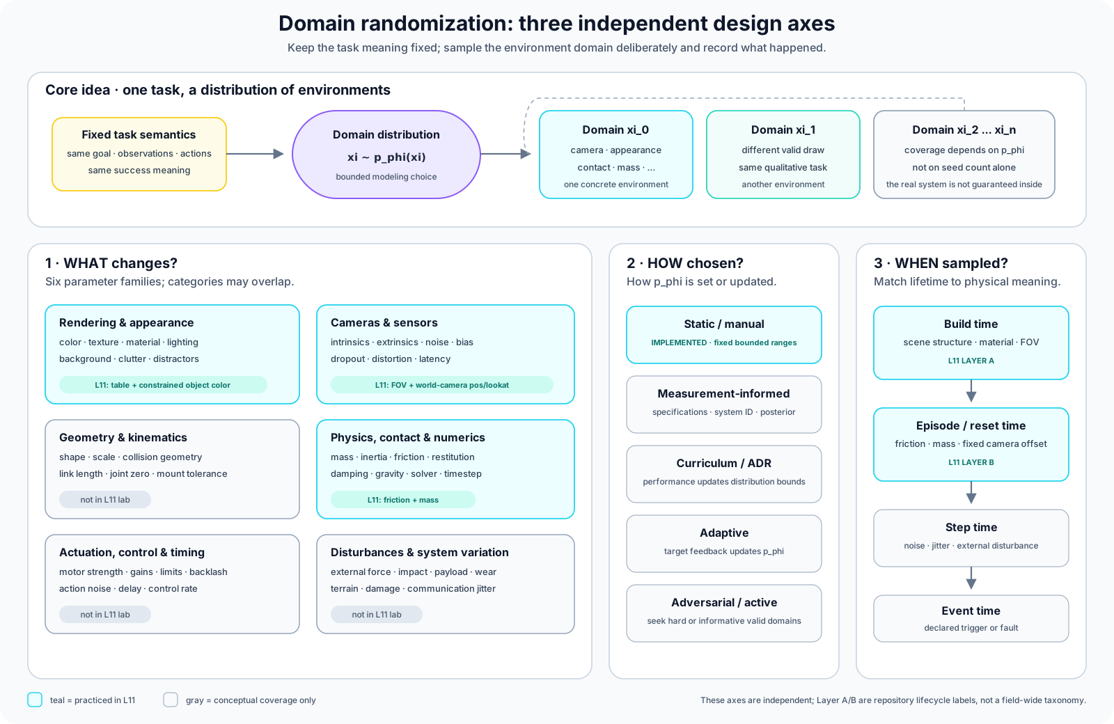
Course-created diagram. It separates what is randomized from how a domain is selected and when its values are sampled. Highlighted items form this lesson's practical subset, not a claim of complete coverage.

Why randomize at all?

A learner can exploit any stable shortcut in a simulator. A vision model might associate the target with one exact table color or camera framing. A controller might depend on one friction coefficient, one latency, or a numerical artifact of the physics engine. The shortcut may perform well in the nominal simulator and disappear under a slightly different simulator or physical robot.

Domain randomization acts as regularization over environments: a feature or behavior useful across many sampled domains is less tied to one nominal model. From a probabilistic viewpoint, the distribution represents uncertainty about the target environment. Neither view says that more randomness is always better. Irrelevant variation wastes data; implausible variation can destabilize simulation or teach an unnecessarily conservative policy.

Domain randomization is not a transfer certificate

Different-looking images show that a rendering knob changed. Finite rollouts show that sampled simulations remained numerically usable. Neither result establishes better policy performance. A sim-to-real claim requires a frozen training protocol and evaluation on the physical target system.

What can be randomized?

There is no single universally mandated list. A useful robotics taxonomy asks which part of the data-generating and control process is uncertain.

Family	Representative parameters	Gap being modeled	L11 lab coverage
Rendering and appearance	color, texture, material, roughness, metallic/specular response, lights, shadows, background, clutter, distractors	simulated versus deployed visual appearance	table color and constrained object color only
Cameras and sensors	intrinsics, extrinsics, FOV, distortion, exposure, blur, RGB/depth noise, dropout, bias, drift, quantization, latency; proprioceptive, force/torque, or tactile noise	idealized versus physical sensing	camera FOV and static world-camera pose
Geometry and kinematics	object shape/scale, collision geometry, link length, joint zero/range, camera-mount tolerance, terrain geometry	CAD, calibration, manufacturing, and assembly error	not implemented as DR
Physics, contact, and numerics	mass, inertia, center of mass, friction, restitution, compliance, damping, gravity, contact model, solver settings, timestep	model and parameter error in transitions	shared friction ratio and per-object mass ratio
Actuation, control, and timing	motor strength, efficiency, gear ratio, controller gains, limits, joint friction, backlash, dead zone, action noise, delay, control rate	commanded versus executed behavior	not implemented
Disturbances and system variation	external force/torque, impact, wind, payload, terrain, wear, damage, communication jitter	unmodeled deployment variation	not implemented

The categories overlap because one parameter can change several channels. An object's scale changes both its pixels and its contact geometry. A simulator timestep is a numerical parameter, yet changing the action hold time can also approximate controller latency. World-camera extrinsics belong conceptually to the sensor domain even though this repository changes them at reset time next to physics parameters.

Visual randomization is only one branch

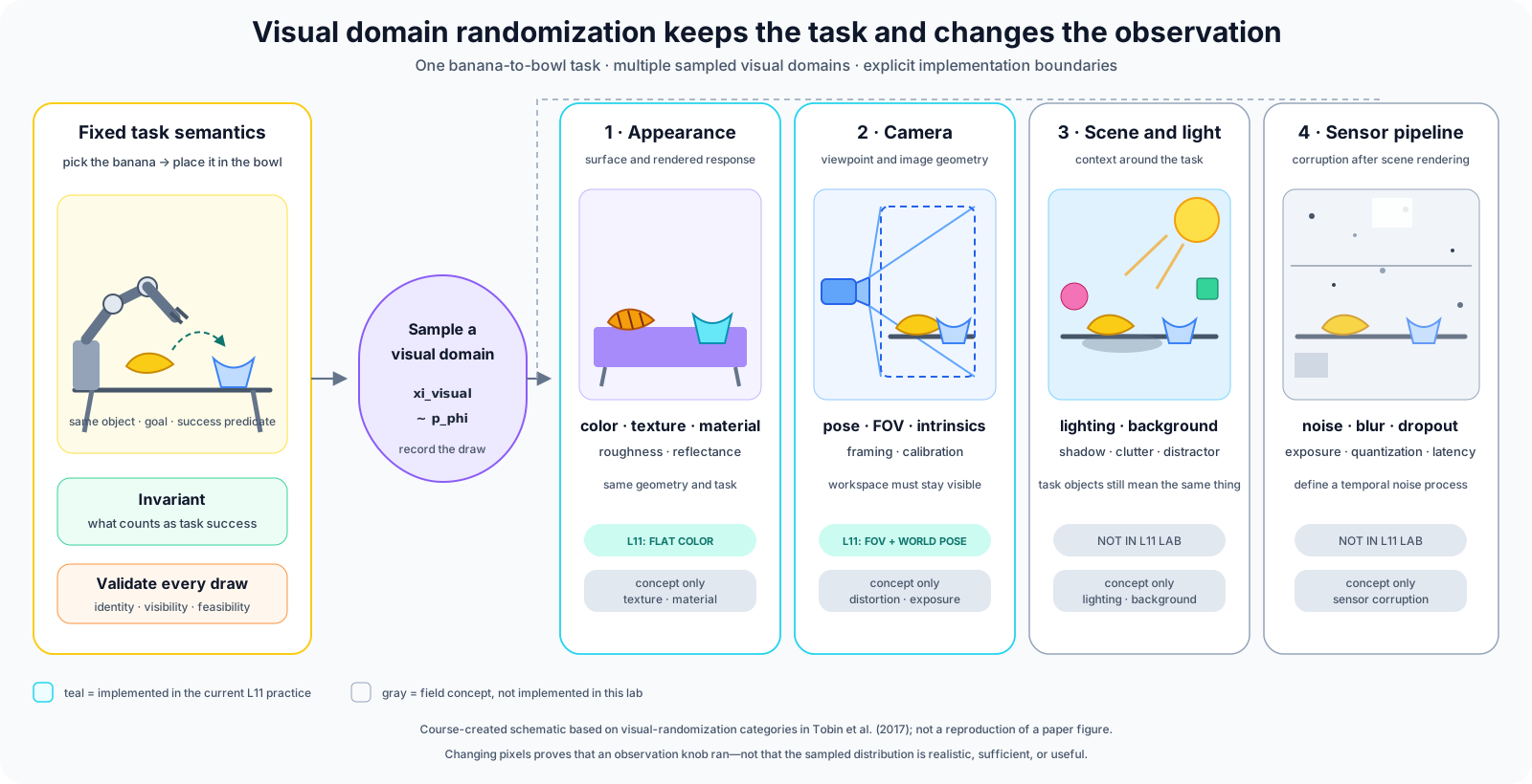
Course-created schematic based on the visual-randomization categories in Tobin et al. (2017); it is not a reproduction of a paper figure. The scene cards build intuition about observation changes, not evidence that the current simulator implements every depicted parameter.

Tobin et al. randomized object and background textures, object and camera poses, field of view, lights, distractors, and image noise for simulated-to-real object localization. That influential example explains why DR is often introduced visually, but it does not bound the field.

This repository currently randomizes color, not texture. When object recolor is enabled, build_scene() replaces the original mesh texture with a flat-color surface drawn from an object-specific HSV prior. It does not sample texture maps, material roughness, lighting, or backgrounds. Calling that implementation "texture randomization" would overstate what the code does.

Dynamics randomization reaches the control loop

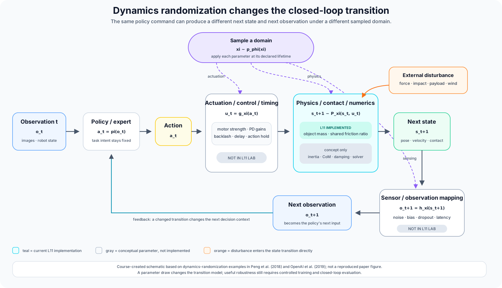
Course-created control-loop schematic based on dynamics-randomization examples in Peng et al. (2018) and OpenAI et al. (2019); it is not a reproduction of a paper figure. Teal marks the current lab implementation, while gray and orange parameters remain conceptual here.

Peng et al. demonstrated a much broader dynamics vector: robot-link and object mass, damping, friction, table height, position-controller gains, the time between actions, and observation noise. OpenAI's dexterous manipulation work additionally included geometry, actuator properties, backlash, latency, observation corruptions, visual parameters, and disturbances.

These examples reveal why friction + mass is a useful experiment but not a complete definition of dynamics randomization. A real control stack also has calibration error, saturation, bandwidth, delay, quantization, and correlated noise. Which parameters matter is task- and platform-dependent.

Keep the task boundary explicit

Domain randomization normally seeks one policy or model that solves the same qualitative task across different environments. The boundary is operational, not a property of a parameter name.

For example, object position can mean different things:

• for "locate a banana anywhere on this work surface," position is a domain variation inside one task;
• for a benchmark with a prescribed initial state, changing position creates a different task instance; and
• moving the goal from a bowl to an arbitrary shelf can change both task semantics and difficulty.

This course uses the following convention so that evidence remains auditable:

Concept	What changes	Course example	Main question
Task randomization	initial condition, goal, or task instance	object xy/yaw, selected pick object, place target	Is the requested task still the same instance and difficulty?
Domain randomization	observation, transition, actuation, timing, or disturbance domain	color, FOV, friction, mass, camera pose	Does the same task survive plausible deployment variation?
Data augmentation	an already generated sample	crop, color transform, or image noise after reading	Does the transform preserve the sample's semantics?
System identification	an estimate of real parameters or uncertainty	infer mass, friction, or latency from trajectories	Which simulator settings best explain measurements?
Domain adaptation	a representation, model, or simulator aligned with target data	align simulated and real image features	How is target-domain information used to reduce mismatch?

The literature sometimes draws these borders differently. In a broad MDP formulation, initial states and goals can be included in the domain parameters. Some visual-DR systems also include online image distortions that this course would call data augmentation. State the convention and the stage at which a transformation occurs instead of arguing that one label is universally correct.

Three independent design axes

The six families answer what changes. Two more questions define a DR scheme: how the distribution is chosen and when a sample is applied. Mixing these axes leads to statements such as "camera pose is dynamics" merely because it is updated beside mass at reset.

How is the domain distribution chosen?

Muratore et al. organize the algorithmic landscape around static, adaptive, and adversarial randomization. For this lesson, the following map is more useful than one long algorithm list:

Strategy	Distribution behavior	Information required	Course depth
Static/manual DR	Hand-designed ranges remain fixed	engineering judgment, specifications, or prior experiments	implemented and inspected
Measurement-informed DR	Measurements or system identification set nominal values and uncertainty	target-system observations	conceptual connection
Curriculum / automatic DR	Bounds grow or shrink with model performance	training-time performance at sampled boundaries	conceptual overview
Adaptive DR	The distribution is updated to reduce simulated/target trajectory mismatch	target-domain data and an update rule	conceptual overview
Adversarial / active DR	Sampling seeks difficult or informative valid domains	an adversary, acquisition objective, or robustness criterion	conceptual overview

OpenAI's automatic domain randomization (ADR), for example, begins with narrow ranges and adjusts individual boundaries according to performance. That is a method for changing p_phi(xi) during training; it is not a new family of physical parameters.

The common independent-uniform design is convenient:

friction_ratio ~ Uniform(low_friction, high_friction)
mass_ratio     ~ Uniform(low_mass, high_mass)

It can still be a poor model. Real parameters may be correlated, conditional, skewed, or multimodal. Camera exposure and illumination are related; payload and center of mass are related; a larger object may require a different valid initial pose. A distribution that samples every knob independently can create combinations that are individually legal but jointly impossible.

When should a value be sampled?

Lifetime	Appropriate examples	Invariant to preserve
Build time	mesh/material choice, geometry, parameters that Genesis fixes before scene.build()	one built scene keeps its declared structure
Episode/reset time	mass, friction, fixed calibration offsets	the physical device does not change identity halfway through a trajectory
Step time	uncorrelated sensor noise, action noise, communication jitter, external disturbances	fast variation follows an explicit stochastic process
Event time	impact-dependent perturbation, a declared fault or payload event	the trigger and state transition are recorded

Sampling frequency follows physical meaning, not convenience. Resampling mass, object size, or a bolted camera pose every frame creates a different and often unphysical system. Sampling one value of white sensor noise at build time does not model frame-to-frame noise.

Choose ranges that preserve a usable task

A DR distribution should be wide enough to cover relevant uncertainty and narrow enough to preserve physical feasibility and task meaning. Before collecting data, check each proposed range against four constraints:

1. Semantic validity: the object, observation, instruction, and success predicate still refer to the same task.
2. Physical validity: masses remain positive, geometry does not intersect, camera frusta cover the workspace, and solver inputs remain finite.
3. Operational validity: the expert or learning process can encounter the condition without the dataset collapsing to almost no accepted examples.
4. Target relevance: the range represents a stated uncertainty or stress condition, rather than variation added only because a knob exists.

Start narrow and isolate one factor

Hold task pose and other domain parameters fixed, change one family, inspect the sampled values and observations, and only then compose factors. This does not prove the final distribution is optimal, but it makes configuration bugs and confounding much easier to see.

Wider is not automatically better. An excessively broad distribution can make the simulator unstable, destroy visual identity, increase expert failures, or force a policy to spend capacity on irrelevant extremes. An excessively narrow distribution may add noise without covering the target variation. The chosen ranges therefore belong in experiment provenance, not only in source-code defaults.

This course implements a deliberate subset

The field taxonomy tells us what could be modeled. The repository's Layer A and Layer B tell us when Genesis can apply the selected subset.

Course layer	Sampling boundary	Implemented parameters	Important omissions
Layer A	before scene.build()	table RGB, constrained object RGB, world/wrist/video vertical FOV	textures, materials, lighting, backgrounds, geometry
Layer B	each EnvRandomizer.reset()	shared contact-surface friction ratio, per-object mass ratio, static world-camera pos/lookat	inertia/CoM, damping, restitution, robot morphology, actuator/timing and sensor noise

This is an implementation lifecycle, not a universal DR taxonomy. Layer B is named for the runtime path, but its camera extrinsics remain an observation-side parameter. The two layers can be composed; that does not make their effects statistically independent.

Layer A: build-time appearance and intrinsics

SceneDomainRandomizationConfig is passed to build_scene() before the scene is built:

from robo_genesis.build_scene import SceneDomainRandomizationConfig, build_scene

scene_dr = SceneDomainRandomizationConfig(
    enabled=True,
    table_color_jitter=0.15,
    randomize_object_color=True,
    fov_jitter_deg=2.0,
    seed=0,
)
bundle = build_scene(scene_dr=scene_dr)

One NumPy RNG stream, initialized from scene_dr.seed, determines all Layer-A draws for that build.

Table color

The table top and legs start from their configured RGB values. Each channel receives an independent uniform offset in [-table_color_jitter, +table_color_jitter], then is clipped to [0, 1]. Clipping makes the output legal but can concentrate samples at zero or one when the amplitude is too large.

Constrained object recolor

Only objects listed in DR_APPEARANCE_PRIORS are recolored. Their hue, saturation, and value are sampled inside object-specific intervals, then converted to RGB. The prior is a semantic guardrail: a banana should remain recognizable as the intended object rather than become an arbitrary color.

The current surface is flat color. It replaces the original mesh texture and does not synthesize a new texture. That limitation should remain visible when interpreting a montage.

Camera FOV

The configured vertical FOV of each created camera receives its own uniform offset in [-fov_jitter_deg, +fov_jitter_deg]. FOV is an intrinsic camera parameter: it changes framing without moving the camera center. A safe configuration keeps every resulting FOV positive and keeps the manipulation workspace visible.

These values are fixed by the current build path. A new Layer-A sample requires a new scene and therefore pays the scene.build() cost.

Layer B: reset-time physics and world-camera pose

DomainRandomizationConfig is nested inside RandomizationConfig and applied by EnvRandomizer.reset():

from robo_genesis.randomize import DomainRandomizationConfig, RandomizationConfig

runtime_dr = DomainRandomizationConfig(
    enabled=True,
    friction_ratio_range=(0.7, 1.3),
    mass_ratio_range=(0.8, 1.2),
    cam_pos_jitter=0.01,
    cam_lookat_jitter=0.02,
)
reset_cfg = RandomizationConfig(
    randomize_pick=False,
    dr=runtime_dr,
)

The numeric intervals above are the current class defaults for friction and mass plus small illustrative camera offsets. They are not universal safe ranges for other robots, objects, solvers, or tasks.

The reset order is deliberate:

restore robot and place objects
  → sample and apply friction + mass
  → settle under the sampled dynamics
  → perturb the static world camera
  → choose the task

Applying dynamics before settling means the initial contacts already use the episode's domain. Moving the camera afterward is safe because it does not alter the physical settle.

Friction belongs to both contact surfaces

L03 established the Genesis 1.3.3 contact-pair rule used here:

effective_pair_friction = max(friction_side_A, friction_side_B)

If only a low-friction object were scaled, unchanged finger or table friction could dominate the maximum. The randomizer therefore applies one shared ratio to the YCB objects, Franka links, and table entities. This is a deliberate implementation for the pinned engine, not a universal friction law for all simulators.

Mass is multiplicative and does not accumulate

For each object, the randomizer captures pristine per-link base mass once and samples a positive ratio:

sampled_mass = base_mass * mass_ratio
mass_shift   = base_mass * (mass_ratio - 1)

An absolute plus or minus kilograms perturbation can make a light object negative. A positive multiplicative ratio preserves sign. Recomputing the shift from the cached base mass also prevents repeated resets from compounding the previous episode's change. Robot mass remains fixed so the tuned Franka gains are not silently reinterpreted.

Only the static world camera moves

cam_pos_jitter and cam_lookat_jitter independently perturb the three coordinates around the configured world-camera baseline. The wrist camera is eye-in-hand and is updated from its attached hand link after each step; its mounting transform is not randomized in this lesson.

The implementation exposes last_friction_ratio and per-object last_mass_ratio for diagnostics. Camera pose and the configuration ranges also need to be recorded if a dataset is to be reproducible.

Seeds must follow the collection transaction

One seed is not enough to identify a recorded episode because the recorder has two schedules and rejects failed attempts.

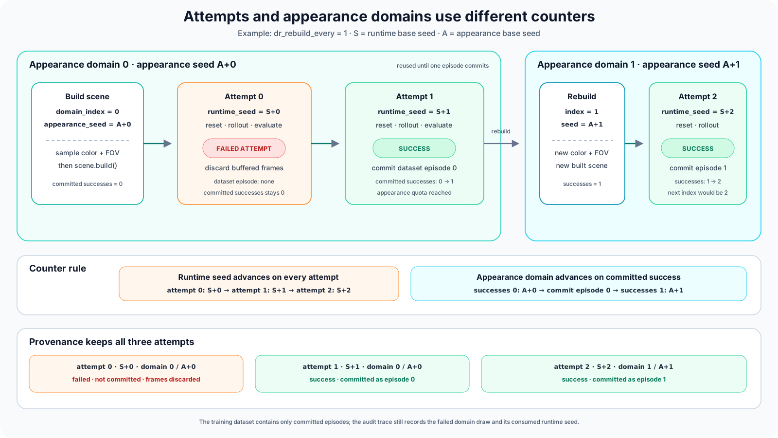
Course-created diagram for dr_rebuild_every=1. Attempt 0 fails and consumes its runtime seed without advancing the appearance domain; attempts 1 and 2 commit episodes 0 and 1, with a rebuild between them.

The current deterministic schedule is:

appearance_base_seed = dr_seed if provided else seed
appearance_domain_index = committed_successes // dr_rebuild_every
appearance_seed = appearance_base_seed + appearance_domain_index

runtime_episode_seed = seed + attempt_index
reset(runtime_episode_seed)

This yields two different counters:

• attempt_index advances after every rollout, whether it succeeds or fails;
• committed_successes advances only after the recorder accepts an episode.

A failed attempt therefore creates a gap in runtime seeds. It does not consume the success quota for the current appearance domain. With dr_rebuild_every=1, the first success triggers the next appearance build, not the first attempt.

Why failed attempts belong in provenance

L09 correctly excludes failed attempts from a success-only demonstration dataset. That transactional rule creates a selection effect under DR: domains in which the scripted expert fails more often contribute fewer or no committed demonstrations. The requested sampling distribution and the distribution observed in the saved dataset may differ.

Saving failed frames as training demonstrations is not the fix. Instead, keep an audit trace outside the standard sample schema. The L11 lab contract uses a course-owned provenance sidecar containing at least:

• schema and implementation version;
• requested ranges and base seeds;
• attempt index and runtime seed;
• appearance-domain index and seed;
• actual friction, per-object mass ratios, and world-camera pose;
• success/commit outcome; and
• committed episode index when one exists.

The preferred location is meta/robo_genesis_domain_randomization.json if LeRobot finalization preserves an additional course-owned metadata file. Otherwise the recorder must use an explicit sibling provenance path. It must not mutate the standard LeRobot feature schema or hide provenance only in a directory name.

Current implementation boundary

The existing recorder already implements the two seed schedules and DR knobs, but the L11-specific validation and provenance sidecar are part of the companion-lab implementation contract. Until that work is complete and verified, console output or a directory named dr is not equivalent to a machine-readable audit trail.

Split by episodes and account for domains

L10 rejected random frame splits because neighboring frames from one trajectory would leak across train and evaluation. L11 adds a second grouping variable: the domain.

Evaluation question	Training/evaluation relation	Honest label
Does the policy handle new episodes from the same declared ranges?	disjoint episodes and seeds, same parameter distribution	in-distribution holdout
Does it handle a declared condition absent from training?	held-out seed group, appearance group, or parameter subrange	held-out condition
What happens beyond the training support?	one or more parameters outside the declared training ranges	stress or OOD evaluation

If several consecutive successful episodes share one appearance build, a split by collection order may put an entire appearance group on one side—or split correlated episodes from that group across both sides. Preserve the mapping from episode to appearance domain before selecting IDs.

The lab records four smoke episodes with dr_rebuild_every=2, so their appearance-domain IDs are 0, 0, 1, 1. This small repeated-group structure makes the two split plans visibly different:

Plan	Train episodes	Evaluation episodes	Domain relation
In-distribution	0, 2	1, 3	both sides contain domains 0 and 1
Held-out domain	0, 1	2, 3	domain 0 is train-only; domain 1 is evaluation-only

Four smoke episodes demonstrate grouping and split mechanics. They are still not enough to estimate coverage, compare policies, or form a meaningful benchmark.

Companion lab workflow

The notebook will connect the complete concept to one deliberately small practice path. It does not implement the missing sensor, geometry, actuator, timing, disturbance, or adaptive-distribution families.

Before you run

• Complete L09 first or set the notebook's explicit baseline dataset root to a compatible local copy.
• The normal path uses ROBO_GENESIS_RENDER=1. It builds cameras, renders a fixed-seed preview, records four successful episodes, and reads both videos.
• ROBO_GENESIS_RENDER=0 is a constrained diagnostic. It checks configuration, scheduling, friction/mass arithmetic, and command construction without initializing Genesis or creating a dataset.
• Output roots are resolved explicitly. An existing L11 dataset stops the run unless the exact opt-in overwrite variable is enabled.
• The lab does not scan arbitrary directories, download a fallback dataset, or commit generated images, videos, caches, or provenance files.

Step 1: predict before rendering

Start with a baseline and change only one factor. Before seeing an image, state:

• which technical family the factor belongs to;
• whether it needs a build or a reset;
• which camera observations it can change;
• whether it can affect expert success; and
• what value and seed must appear in provenance.

This separates causal reasoning from visual guesswork.

Step 2: render fixed Layer-A domains

The current preview tool creates a DR-off baseline and one process per requested appearance seed:

.venv/bin/python -m robo_genesis.tools.dr_preview \
  --seeds 0 1 \
  --object-color \
  --table-jitter 0.15 \
  --fov-jitter 2.0 \
  --output-dir outputs/eval_results/l11_dr_preview

Use --cpu only when intentionally testing the CPU backend. The generated world frames should be readable, finite, non-empty, and visibly preserve the task workspace. A different image establishes that the active knobs changed rendered observations; it does not establish sufficient or useful coverage.

Step 3: inspect Layer-B guardrails

Before running a full scene, the notebook reproduces two small calculations:

1. the Genesis contact-pair max() rule, showing why scaling only the object can be masked by the finger or table; and
2. multiplicative mass scaling, showing why positive ratios avoid negative masses and why every reset must reference the pristine base mass.

The full path then reads the actual sampled ratios and camera pose from the runtime objects. Reimplementing a second random sampler in the notebook would only test the notebook against itself.

Step 4: record a four-episode combined smoke

The compact experiment uses:

Setting	Lab value	Reason
Successful episodes	4	gives each of two appearance domains two episodes
Maximum attempts	10	bounded failure behavior
Dataset FPS	5	matches the small L09 baseline
Image size	640×360	restores the recorder's default 16:9 output for a clearer visual review
Pick task	banana to bowl	preserves the L09 comparison
Layer-A rebuild interval	2 accepted episodes	makes both in-domain and held-out-domain splits observable
Layer B	bounded friction, mass, and world-camera jitter	tests the current runtime subset

An explicit command equivalent to the notebook's subprocess is:

.venv/bin/python -m robo_genesis.record_dataset \
  --episodes 4 \
  --max-attempts 10 \
  --seed 1100 \
  --fps 5 \
  --img-width 640 \
  --img-height 360 \
  --vcodec h264 \
  --pick 011_banana \
  --repo-id local/l11_banana_dr \
  --output-dir datasets/l11_banana_dr \
  --dr-appearance \
  --dr-object-color \
  --dr-table-jitter 0.15 \
  --dr-fov-jitter 2.0 \
  --dr-rebuild-every 2 \
  --dr-runtime \
  --dr-friction 0.7 1.3 \
  --dr-mass 0.8 1.2 \
  --dr-cam-pos 0.01 \
  --dr-cam-lookat 0.02

The lab stops rather than overwriting an existing root unless the learner explicitly opts in, and it fails clearly if ten attempts do not produce the four requested successes. These safeguards have been verified against the final recorder implementation.

Step 5: audit data and provenance together

Reopen the L09 baseline and L11 DR dataset with LeRobot 0.6.0. For both, report the exact root, logical repository ID, schema version, FPS, episode/frame counts, camera keys, image shapes, and codec. Decode synchronized world/wrist frames from identified episodes rather than comparing anonymous screenshots.

Then join each committed L11 episode with the provenance trace. The audit must be able to answer:

• Which attempt produced this episode?
• Which runtime and appearance seeds were used?
• Which actual physics and camera values were sampled?
• Which failed attempts occurred before it?
• Did two split groups accidentally share an appearance domain?

A descriptive per-episode image statistic may accompany the frames, but no four-episode statistic should be called a diversity, generalization, or robustness result.

Evidence ladder

Evidence	What it establishes	What it does not establish
A fixed seed reproduces one configuration and preview	configuration and seed path are traceable	pixel-identical rendering across all platforms
Baseline and sampled-domain images differ	selected knobs affect rendered observations	realism, sufficient coverage, or policy benefit
Ratios and poses are finite and inside bounds	the Layer-B application path is usable	monotonic contact or grasp difficulty
Four successful DR episodes reopen with both videos	recorder, writer, codec, sidecar, and reader connect; repeated domain groups make split mechanics visible	adequate data or training convergence
Attempt and success counts agree with provenance	the smoke run's selection is observable	population expert success rate
A frozen policy improves on a declared simulated holdout	evidence for that simulator protocol	real-world transfer
A frozen policy improves on a physical robot protocol	evidence for that robot, task, and condition set	universal robustness

The lesson ends at dataset and provenance evidence. L12 trains policies; L13 performs closed-loop evaluation. Do not move claims upward in this ladder.

Diagnose failures by boundary

1. Baseline dataset missing: print the exact root. Run L09 or provide one compatible local root; do not scan unrelated directories or download an unknown replacement.
2. Output already exists: stop by default. Enable overwrite only after confirming the exact L11 target directory.
3. Preview does not change: check enabled, non-zero knobs, seeds, and whether a fresh scene was actually built.
4. Object appearance is implausible: check that the object has a DR_APPEARANCE_PRIORS entry and remember that flat recolor replaces its original texture. Do not widen hue arbitrarily.
5. The task leaves the image: isolate FOV from camera-pose jitter, reduce the range, and inspect the work surface in actual world-camera frames.
6. Friction appears unchanged: check the object, contacting Franka links, and table all receive the shared ratio before reasoning about motion.
7. Mass causes NaN or drift across resets: require a positive ratio and recompute the shift from the cached pristine mass rather than the last episode's mass.
8. The same seed appears different: compare backend, code and asset versions, appearance-domain index, attempt history, and the complete config. A seed is not an environment identity by itself.
9. A requested domain is absent from saved data: inspect failed-attempt provenance and the success gate before blaming the reader.
10. Evaluation is unexpectedly strong or weak: inspect episode/domain leakage and whether a whole appearance group landed on one side before changing the policy.

Checkpoints and one-variable exercise

Concept checkpoints

1. Why is DR a distribution over environments rather than a list of recorder flags?
2. For one proposed parameter, does it mainly change observation, physics, actuation/timing, or disturbance? Can it affect more than one?
3. Why are Layer A and Layer B repository lifecycle labels rather than a general robotics taxonomy?
4. Why can object pose be task randomization in one experiment and domain variation in another?
5. How do data augmentation, system identification, and domain adaptation differ from DR, and how can they complement it?
6. Why should mass normally remain fixed within a trajectory while independent sensor noise can change every step?
7. Why do failed attempts consume runtime seeds but not appearance-domain success quotas?
8. Why can a success-only recorder distort the requested domain distribution?
9. Why do two different images or a larger RGB spread fail to prove policy robustness?
10. What additional protocol and evidence would be required for a sim-to-real claim?

One-variable exercise: isolate a domain parameter

Return to l11-appearance-preview in notebook Section 2. Change only PREVIEW_PROFILE from combined to table_color, object_color, or fov, then rerun Sections 2 and 3. Each profile fixes the unselected knobs at zero, keeps seeds 0 and 1, and writes into an isolated preview subdirectory. Runtime world-camera pose is deliberately excluded: it is a reset-time Layer-B parameter and requires episode recording rather than this quick build-time preview.

Before running, predict:

• its technical family;
• its build/reset sampling boundary;
• which observation should change;
• whether it can affect task validity or expert success; and
• which requested and actual values must be recorded.

After running, compare the prediction with labeled frames and provenance. State only what the evidence shows. Do not conclude that the changed parameter improves a policy without a controlled training and closed-loop evaluation.

Summary

• Domain randomization samples a distribution of environment parameters while preserving the qualitative task; it is not synonymous with visual noise or recorder flags.
• Robotics DR can cover rendering, sensors, geometry, physics, actuation, timing, and disturbances. What changes, how domains are selected, and when values are sampled are separate design axes.
• Static manual DR is only one strategy. Measurement-informed, automatic, adaptive, and adversarial methods change how the domain distribution is chosen, not which physical category a parameter belongs to.
• This course deliberately practices a smaller subset: build-time color/FOV and reset-time friction/mass/world-camera pose. It does not implement texture, lighting, sensor noise, geometry, actuator, or disturbance randomization.
• Seeds, requested ranges, actual draws, failed attempts, and commit decisions are part of the data's identity. A success-only dataset can differ from the requested randomization distribution.
• A valid preview and readable smoke dataset establish an implementation path, not policy robustness or sim-to-real transfer.

Sources

• Muratore et al., “Robot Learning From Randomized Simulations: A Review” — domain-parameter formulation, practical randomization considerations, and the static/adaptive/adversarial taxonomy.
• Tobin et al., “Domain Randomization for Transferring Deep Neural Networks from Simulation to the Real World” — visual randomization over textures, scene objects, cameras, lights, and image noise.
• Peng et al., “Sim-to-Real Transfer of Robotic Control with Dynamics Randomization” — randomized dynamics, controller timing, and observation noise for robotic control.
• OpenAI et al., “Solving Rubik's Cube with a Robot Hand” — automatic domain randomization and a broad simulator-physics, custom-physics, observation, vision, and disturbance parameter set.
• Genesis World documentation and Genesis World 1.3.3 on PyPI — official engine/API documentation and the exact version pinned by this course.
• Genesis 1.3.3 RigidEntity source and rigid-contact implementation — version-pinned runtime mass/friction APIs and contact-pair behavior.
• Genesis 1.3.3 Camera source — version-pinned camera construction, FOV, pose, attachment, and rendering behavior.
• RoboGenesis 101 scene builder, environment randomizer, dataset recorder, and DR preview tool — the current Layer-A/Layer-B behavior and collection schedule used by this lesson.