Chapter 14: Reinforcement Learning with Verifiable Rewards (RLVR)

In previous courses, we discussed RLHF (Reinforcement Learning from Human Feedback). Although RLHF is key to making models follow instructions, it faces enormous scalability challenges: human feedback is expensive, slow, and easily "over-optimized" (Goodhart's Law).

In this chapter, we turn our attention to the core technology behind reasoning models like o1 and DeepSeek R1—RLVR (Reinforcement Learning from Verifiable Rewards).

Core objectives:

1. Algorithm evolution: Understand the logic of evolution from PPO to GRPO, and why GRPO is more suitable for large model reasoning training.
2. Engineering implementation: Delve into the code implementation details of PPO and GRPO, master Advantage calculation and Loss design.
3. Frontier cases: Deconstruct the training pipelines of DeepSeek R1, Kimi k1.5, and Qwen 3, understand the key roles of "cold-start data," "Chain of Thought (CoT)," and "length control."

14.1 Why Do We Need RLVR?

In fields like AlphaGo or AlphaFold, reinforcement learning has achieved great success because they have perfect simulators and explicit reward functions (win/loss, protein folding energy levels).

In language models, if we can find similar domains—where answers are objective and verifiable (e.g., math problems, code generation)—we can use large-scale computing resources to replace expensive human annotation, and let the model evolve through reinforcement learning. This is the core vision of RLVR.

14.1.1 The Predicament of RLHF

Traditional RLHF relies on humans making pairwise preference judgments on model outputs (e.g., "A is better than B"). However, this approach has three fundamental problems:

• High reward noise: Human judgments are subjective, inconsistent, and easily misled by surface rhetoric;
• Difficult to scale: High-quality preference data annotation costs are extremely high, unable to support trillion-token-level training;
• Over-optimization: The model learns to "please" the reward model, generating outputs that seem reasonable but are hollow, verbose, or even hallucinatory.

RLHF optimizes a proxy objective (human preferences), not the true objective (task correctness).

14.1.2 Lessons from Success Stories

Looking at successful RL cases like AlphaGo and AlphaFold, their common point is: the reward function is explicit, verifiable, and automatically computable. For example:

• Go: Whether the game is ultimately won (0/1);
• Protein folding: The RMSD (Root Mean Square Deviation) distance between the predicted protein structure and the true structure.

In such tasks, the RL algorithm can directly optimize the true objective without human intermediation. This inspires us: Can RL be introduced into the "verifiable tasks" of language models?

14.1.3 The Positioning of RLVR

RLVR focuses on a special class of tasks: outputs that can be automatically scored by programs. Typical scenarios include:

• Mathematical reasoning: Whether the answer matches the standard solution (e.g., GSM8K, MATH);
• Code generation: Whether the generated program passes all test cases;
• Formal proofs: Whether the proof steps are logically self-consistent.

In these scenarios, the reward function $R(z)$ can be defined as:

$$R(z)=\{\begin{array}{ll}1& \text{if }z\text{ is correct}\\ 0& \text{otherwise}\end{array}$$

Or more refined process rewards (e.g., score per reasoning step). This high signal-to-noise ratio, scalable reward is exactly the stage for RL to shine.

✅ The essence of RLVR: In those narrow-domain tasks where "right and wrong can be automatically determined," bypassing human preferences and directly using formal verification mechanisms to provide reinforcement learning's reward signal, thereby achieving more reliable, scalable, and verifiable agent training

Below is a simple comparison of RLHF and RLVR:

Dimension	RLHF	RLVR
Reward source	Human preferences (e.g., ranking)	Automatic verification (e.g., tests, proofs, rules)
Task domain	General, open-domain (e.g., chat)	Narrow, structured (e.g., programming, math)
Reward quality	Subjective, noisy, expensive	Objective, precise, scalable
Alignment goal	"Makes people feel good"	"Correct in the formal sense"

14.2 Algorithm Evolution: From PPO to GRPO

To understand the GRPO algorithm behind current reasoning models like DeepSeek-R1, we must first review its predecessor PPO, and understand why it was abandoned.

14.2.1 PPO

Development Trajectory of Policy Optimization Methods in RL

From the original Policy Gradient → to the more stable TRPO (Trust Region Policy Optimization) → to the more practical PPO (Proximal Policy Optimization)

In reinforcement learning, we have a policy ${\pi }_{\theta }(a|s)$, which uses parameters $\theta$ to control how the agent chooses action $a$ given state $s$.
The goal is: maximize the expected return:

$$J(\theta )={\mathbb{E}}_{\tau \sim {\pi }_{\theta }}[R(\tau )]$$

Where $\tau =(s_1,a_1,s_2,a_2,...,s_T)$ is a trajectory, and $R(\tau )$ is the total reward.

We need to compute ${\mathrm{\nabla }}_{\theta }J(\theta )$ to update $\theta$ via gradient ascent.

🔹 Attempt 1: Policy Gradient

Using the likelihood ratio trick, we can derive:

$${\mathrm{\nabla }}_{\theta }J(\theta )={\mathbb{E}}_{\tau \sim {\pi }_{\theta }}[R(\tau ){\mathrm{\nabla }}_{\theta }\log {\pi }_{\theta }(\tau )]$$

And ${\pi }_{\theta }(\tau )=p(s_1)\prod _{t=1}^T{\pi }_{\theta }(a_t|s_t)p(s_{t+1}|s_t,a_t)$, so ${\mathrm{\nabla }}_{\theta }\log {\pi }_{\theta }(\tau )=\sum _{t=1}^T{\mathrm{\nabla }}_{\theta }\log {\pi }_{\theta }(a_t|s_t)$

Thus we get the REINFORCE algorithm (the most basic policy gradient):

$${\mathrm{\nabla }}_{\theta }J(\theta )={\mathbb{E}}_{\tau \sim {\pi }_{\theta }}[\left(\sum _{t=1}^T{R}_t\right)\sum _{t=1}^T{\mathrm{\nabla }}_{\theta }\log {\pi }_{\theta }(a_t|s_t)]$$

Where $R_t=\sum _{k=t}^T{\gamma }^{k-t}{r}_k$ is the discounted return from time $t$.

What problems does policy gradient have:

• High variance: Because the total reward $R(\tau )$ of the entire trajectory is used as the "signal" for each action, but many actions are actually unrelated to the final result.
• Unstable updates: One update may be too large, leading to policy collapse ("catastrophic collapse").

✅ So policy gradient is theoretically correct, but practically difficult to use.

🔹 Attempt 2: TRPO (Trust Region Policy Optimization)

Core idea: Instead of using raw gradient updates directly, allow the policy to change only a little each time, ensuring the new policy ${\pi }_{{\theta }_{\text{new}}}$ and the old policy ${\pi }_{{\theta }_{\text{old}}}$ are close enough.

Specific approach: Solve a constrained optimization problem:

$$\begin{gathered} \underset{\theta }{max}{\mathbb{E}}_{s,a\sim {\pi }_{{\theta }_{\text{old}}}}[\frac{{\pi }_{\theta }(a|s)}{{\pi }_{{\theta }_{\text{old}}}(a|s)}{A}^{{\pi }_{\text{old}}}(s,a)] \\ \text{subject to}{\mathbb{E}}_s\left[D_{\text{KL}}({\pi }_{{\theta }_{\text{old}}}(\cdot |s)\parallel {\pi }_{\theta }(\cdot |s))\right]\le \delta \end{gathered}$$

• This objective approximately improves the policy (using importance sampling + advantage function $A$)
• The constraint limits KL divergence to no more than a small constant $\delta$

TRPO features:

• ✅ Stable, theoretical guarantee of monotonic improvement
• ❌ Extremely complex implementation: requires conjugate gradient or second-order optimization, difficult to scale to large models (e.g., LLM)

So TRPO is the "ideal but cumbersome" method.

🔹 Attempt 3: PPO (Proximal Policy Optimization)

Motivation: Can we use a simple method to approximate TRPO's "small-step update" idea without solving complex constrained optimization?

PPO's core innovation: Clipped Probability Ratio

Define the probability ratio (likelihood ratio):

$$r_t(\theta )=\frac{{\pi }_{\theta }(a_t|s_t)}{{\pi }_{{\theta }_{\text{old}}}(a_t|s_t)}$$

In TRPO, we want $r_t(\theta )\approx 1$ (i.e., new and old policies output similar probabilities).

PPO's idea: If $r_t(\theta )$ is too large or too small, "clip" it away!

Thus the clipped surrogate objective is proposed:

$$L^{\text{CLIP}}(\theta )={\mathbb{E}}_t[min(r_t(\theta )A_t,\text{clip}(r_t(\theta ),1-ϵ,1+ϵ)\cdot A_t)]$$

Intuitive explanation:

• If $A_t>0$ (this action is good):
  • We want to increase ${\pi }_{\theta }(a_t|s_t)$, i.e., make $r_t>1$
  • But if $r_t>1+ϵ$, the update is too large → clip it, only take $1+ϵ$
• If $A_t<0$ (this action is bad):
  • We want to decrease ${\pi }_{\theta }(a_t|s_t)$, i.e., make $r_t<1$
  • But if $r_t<1-ϵ$, the penalty is too harsh → clip it to $1-ϵ$

🎯 In this way, PPO automatically limits the step size of policy updates without explicit KL constraints!

🔁 Summary of the Three

Method	Core Idea	Whether to Constrain Update Step	Implementation Difficulty	Suitable for LLM?
Policy Gradient	Direct gradient ascent	❌ No	Simple	❌ (high variance)
TRPO	Constrain updates with KL divergence	✅ Yes (hard constraint)	Extremely difficult	❌ (high memory/computation)
PPO	Approximate small-step updates with clipping	✅ Yes (soft constraint)	Moderate	✅ (mainstream choice)

PPO's Pain Points

The figure below shows the overall process of training a language model using the Proximal Policy Optimization (PPO) algorithm in Reinforcement Learning from Human Feedback (RLHF).

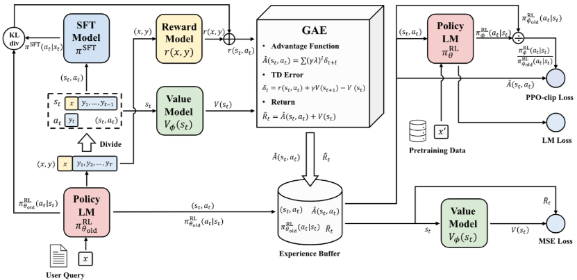
Figure 14.0 PPO algorithm flow chart

The process starts with a user query $x$, the old policy model (Policy LM) generates a response sequence $y_1,y_2,...,y_{t-1}$ based on the input $x$. $(x,y)$ is decomposed into state-action pairs $(s_t,a_t)$. In the language model:

• State $s_t$ = current context (e.g., already generated partial tokens)
• Action $a_t$ = the next token to generate

The user question + model generated answer (x, y) is fed into the Reward Model, outputting a scalar reward value $r(x,y)$, representing the quality of the answer (higher is better).

The Value Model takes the current state $s_t$ as input, and outputs $V(s_t)$, which is the estimate of the total return (Return) from that state.

The Generalized Advantage Estimation (GAE) module computes the advantage $A(s_t,a_t)$ and the estimated return $R{̂}_t$.

Return: $R{̂}_t=Â(s_t,a_t)+V(s_t)$

Advantage Function: $Â(s_t,a_t)=\sum (\gamma \lambda {)}^l{\delta }_{t+l}$, which is a weighted sum of TD errors over future time steps, where $\lambda$ is a GAE parameter (controlling the bias-variance trade-off).

Temporal Difference Error (TD Error): ${\delta }_t=r(s_t,a_t)+\gamma V(s_{t+1})-V(s_t)$, which measures the gap between "actual return" and "current value estimate."

• $r_t$: the immediate reward obtained after executing action $a_t$ in state $s_t$
• $\gamma \in [0,1]$: discount factor, usually taken as 0.95~1.0
• $V(s_t)$: the value network's estimate of state $s_t$

The Experience Replay Buffer is used to store data from each rollout, including state-action pairs $(s_t,a_t)$, advantage function estimates $Â(s_t,a_t)$, estimated return $R{̂}_t$, and the action probability under the old policy ${\pi }_{\theta }^{old}(a_t|s_t)$.

The Policy Update Module Policy LM ${\pi }_{\theta }^{RL}(a_t|s_t)$ is the policy model currently being optimized. It takes state $s_t$ as input and outputs the probability distribution of action $a_t$.

PPO-clip Loss is the core loss function of PPO, whose goal is to maximize the expected return (i.e., the score given by the Reward Model) while ensuring stable policy updates.

$${\mathcal{L}}^{\text{CLIP}}(\theta )={\mathbb{E}}_t[min(r_t(\theta )\cdot {\hat{A}}_t,\text{clip}(r_t(\theta ),1-ϵ,1+ϵ)\cdot {\hat{A}}_t)]$$

Where:

• $r_t(\theta )=\frac{{\pi }_{\theta }(a_t|s_t)}{{\pi }_{{\theta }_{\text{old}}}(a_t|s_t)}$: new-old policy probability ratio
• ${\hat{A}}_t$: advantage function computed by GAE (from TD Error)
• $ϵ$: hyperparameter (usually 0.1~0.2), controlling update step size
• clip: clips the ratio to the interval $[1-ϵ,1+ϵ]$

LM Loss is the standard autoregressive language modeling cross-entropy loss, designed to prevent the policy from "forgetting" how to speak human language (catastrophic forgetting) while optimizing rewards.

MSE Loss is the learning objective of the value function, allowing the value network $V_{\varphi }(s_t)$ to accurately predict the expected total return starting from state $s_t$.

PPO-clip Loss decides "where to go" (preference direction), LM Loss ensures "don't go off track" (linguistic reasonableness), MSE Loss provides the "map" (value estimate)—the three work together to let the LLM navigate steadily in the human preference space.

A complete training process should be:

• Sampling phase: Use ${\pi }_{\theta }^{old}$ to generate answer $y$ based on user input $x$ ---> Use Reward Model to score $(x,y)$ as $r(x,y)$ ---> Use Value Model and GAE to compute each token's advantage function $Â(s_t,a_t)$ and return $R{̂}_t$ ---> Store in Experience Buffer.
• Update phase: Sample mini-batch data from Buffer ---> Compute PPO-clip Loss, LM Loss, MSE Loss ---> Backpropagate to update Policy LM and Value Model ---> The updated new policy becomes the next round's ${\pi }_{\theta }^{old}$
• Iteration loop: Repeat sampling → compute reward and advantage → update strategy → new strategy sampling...

When we look at OpenAI's PPO algorithm documentation, it seems very simple:

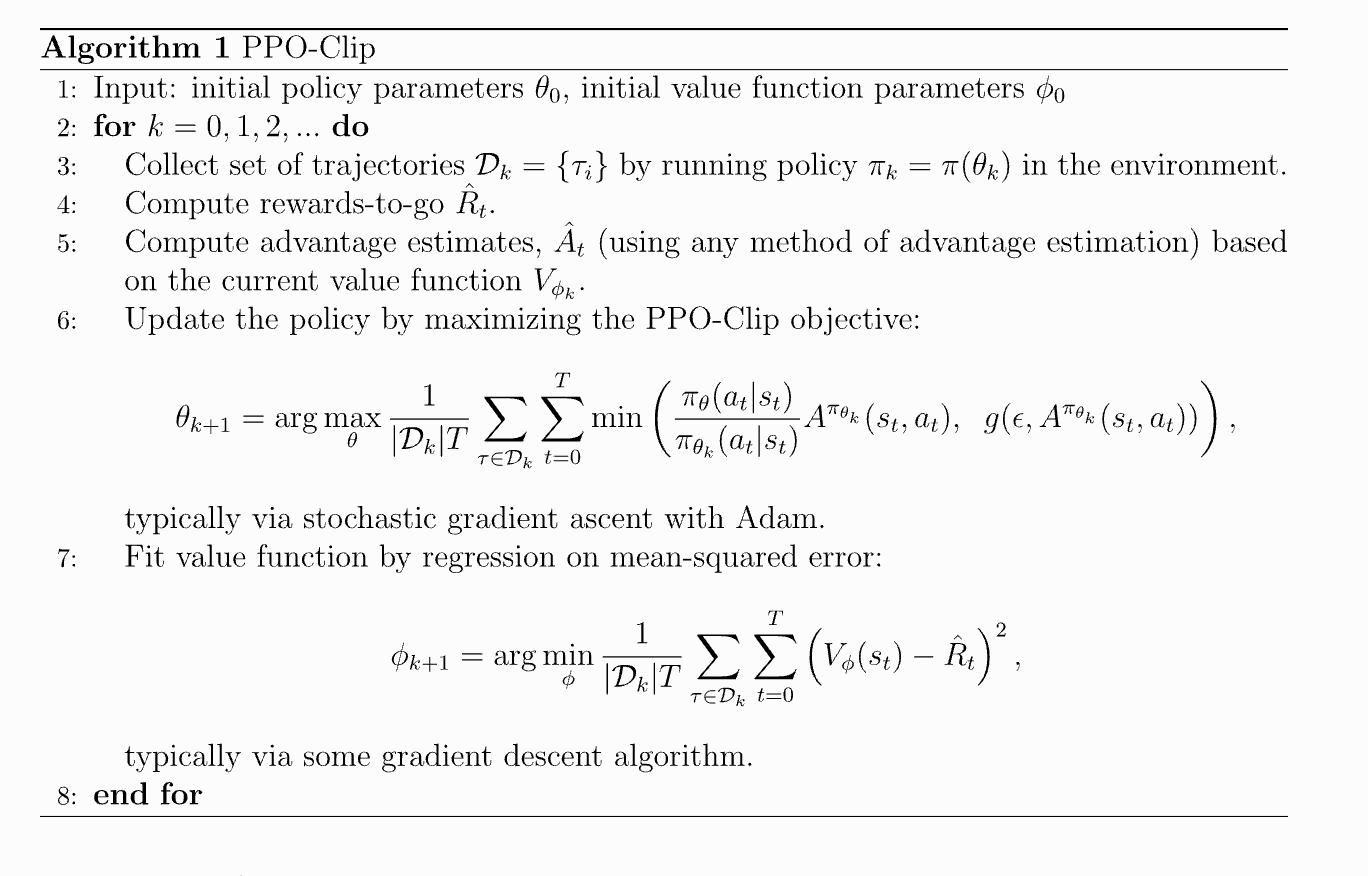
Figure 14.1 PPO algorithm pseudocode

But in practice, the theory and implementation of PPO are two completely different things. PPO theory is concise, but the actual tuning and implementation pitfalls are numerous (such as value function training, advantage estimation, KL control, reward normalization, etc.). There is even a blog listing 37 PPO implementation details, finding that different PPO variants show different scores in RL benchmarks.

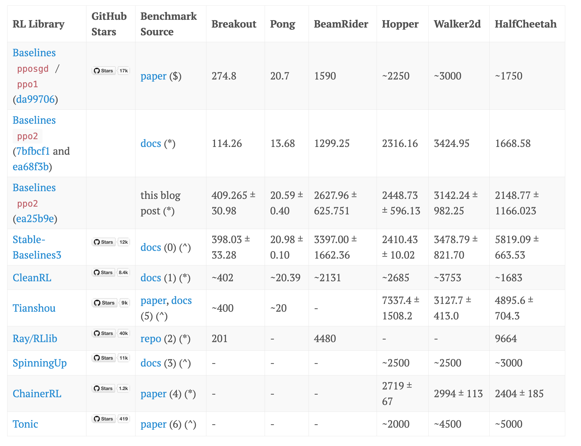
Figure 14.2 Effect of PPO implementation details on performance

And there is a paper that specifically explores why details are so important for PPO, please refer to Implementation Matters in Deep Policy Gradients: A Case Study on PPO and TRPO. And if you really mess them up, even if you don't compute the policy gradient correctly, the effect is actually better. If you look at PPO's implementation details, you'll find the situation is very complex, so we really do need to look at the specific implementation of PPO through code:

Refer to the PPO implementation in alpaca_farm, which follows a typical on-policy RL loop and implements the complete training loop of the PPO algorithm on language models (LLMs), including:

• Rollout (sampling): Use the current policy to generate responses
• Reward calculation and shaping (Reward Shaping): Combine task reward + KL penalty
• Advantage estimation (GAE)
• Loss calculation (Policy + Value Loss with Clipping): Use the PPO loss function to optimize the policy (Actor) and value network (Critic)
• Logging and model saving

Reward Shaping: Combine the sparse task reward (only at the end of the sequence) with the dense KL penalty (every token) to form a trainable reward signal

def _shape_reward(self, rewards, responses, logprobs, ref_logprobs):
    # Compute KL divergence: use only the positive part of (logp - ref_logp) (i.e., penalize only when the new policy is more "confident" than the reference policy)
    kl = torch.clamp(logprobs - ref_logprobs, min=0.0)

    # Non-task reward = -β * KL (β is controlled by self.kl_ctl, can be dynamically adjusted)
    non_score_rewards = -self.kl_ctl.value * kl

    # Initialize shaped rewards: first fill in KL penalty (every token has it)
    shaped_rewards = non_score_rewards.clone()

    # Find the position of the last non-padding token for each sequence (i.e., EOS or actual end)
    terminal_positions = (responses != self.tokenizer.pad_token_id).sum(dim=1) - 1

    # Add the task reward (e.g., whether the math problem is answered correctly) at the last token
    shaped_rewards[list(range(rewards.size(0))), terminal_positions] += rewards

    return dict(shaped_rewards=shaped_rewards, non_score_rewards=non_score_rewards, kl=kl)

Generalized Advantage Estimation (GAE): Use GAE to estimate each token's advantage function, replacing the raw reward, significantly reducing policy gradient variance.

def _estimate_advantage(self, rewards, values):
    if self.args.whiten_rewards:
        rewards = torch_ops.whiten(rewards, shift_mean=False)  # Reward normalization (optional)

    lastgaelam = 0
    advantages_reversed = []
    gen_length = self.args.response_len  # Generation length (e.g., 128)

    # Compute GAE backward (reverse iteration through tokens)
    for t in reversed(range(gen_length)):
        nextvalues = values[:, t + 1] if t < gen_length - 1 else 0.0
        # TD error: δ_t = r_t + γ * V(s_{t+1}) - V(s_t)
        delta = rewards[:, t] + self.args.gamma * nextvalues - values[:, t]
        # GAE: A_t = δ_t + γλ A_{t+1}
        lastgaelam = delta + self.args.gamma * self.args.lam * lastgaelam
        advantages_reversed.append(lastgaelam)

    advantages = torch.stack(advantages_reversed[::-1], dim=1)  # Reverse back to normal order
    returns = advantages + values  # Q(s,a) ≈ A(s,a) + V(s)

    # Advantage function normalization (subtract mean, divide by standard deviation) → reduce variance
    advantages = torch_ops.whiten(advantages, shift_mean=True)

    return dict(returns=returns, advantages=advantages)

rollout (sampling trajectories): Complete a full sampling → evaluation → reward calculation → advantage estimation process, preparing data for subsequent PPO updates

@torch.inference_mode()
def rollout(self, queries_data):
    self.policy.eval()
    unwrapped_policy = self.accelerator.unwrap_model(self.policy, keep_fp32_wrapper=True)
    self.ref_policy.eval()
    self.reward_model.eval()

    rollouts = []
    for batch in tqdm.tqdm(queries_data, desc="rollout"):
        # 1. Generate responses from current policy
        queries, masks = batch['queries'], batch['query_attn_masks']
        responses = unwrapped_policy.respond(queries, masks, temperature=...)  # Generate

        # 2. Use current policy to compute logprobs and values (critic output)
        policy_outputs = self.policy(queries, masks, responses, ...)  # forward

        # 3. Use reference policy (SFT model) to compute ref_logprobs (for KL)
        ref_outputs = self.ref_policy(queries, masks, responses, ...)

        # 4. Convert response to text, then retokenize with reward tokenizer
        #    (because policy and reward model may have different tokenizers)
        text_queries = decode(queries); text_responses = decode(responses)
        text_sequences = [q + r for q, r in zip(text_queries, text_responses)]
        sequences = reward_tokenizer(text_sequences, ...)  # Retokenize

        # 5. Use reward model to compute task reward
        reward_outputs = self.reward_model(**sequences)
        reward_outputs = self.post_reward(reward_outputs, responses)  # Process abnormally ended sequences

        # 6. Reward shaping: add KL penalty
        shaped = self._shape_reward(rewards=reward_outputs['rewards'], ...)

        # 7. Save all data to rollouts
        rollouts_batch.update(policy_outputs, ref_outputs, reward_outputs, shaped)
        rollouts.append(rollouts_batch.cpu())

    # Merge all batches
    rollouts = common.merge_dict(rollouts, merge_fn=torch.cat)

    # 8. Unify GAE calculation (use entire rollout dataset, more stable)
    advantages = self._estimate_advantage(
        rewards=rollouts["shaped_rewards"].to(device),
        values=rollouts["values"].to(device),
    )

    return {**rollouts, **advantages}

PPO loss calculation: Use clipping mechanism to prevent policy updates that are too large

def compute_loss(self, rollouts):
    # Extract old policy data (from rollout)
    values, old_logprob, returns, advantages, ... = rollouts

    # Recompute logprobs and values with current policy
    outputs = self.policy(queries, masks, responses, ...)
    vpred = outputs["values"]      # New value prediction
    logprob = outputs["logprobs"]  # New log prob

    # --- Value Loss (Critic) ---
    # Clip value predictions (similar to PPO clipping)
    vpredclipped = torch.clamp(vpred, values ± cliprange_value)
    vf_losses1 = (vpred - returns) ** 2
    vf_losses2 = (vpredclipped - returns) ** 2
    vf_loss = 0.5 * max(vf_losses1, vf_losses2).mean()  # PPO-style value loss

    # --- Policy Loss (Actor) ---
    ratio = exp(logprob - old_logprob)  # New-old policy probability ratio
    pg_losses = -advantages * ratio
    pg_losses2 = -advantages * clip(ratio, 1-ε, 1+ε)
    pg_loss = max(pg_losses, pg_losses2).mean()  # PPO clipped objective

    # Total loss = policy loss + vf_coef * value loss
    loss = pg_loss + self.args.vf_coef * vf_loss

    # Record statistics
    approxkl = 0.5 * (logprob - old_logprob)^2 的均值
    entropy = outputs["entropies"].mean()

    return loss, stats

In the PPO training process of language models, what does a healthy, reasonable training curve look like?

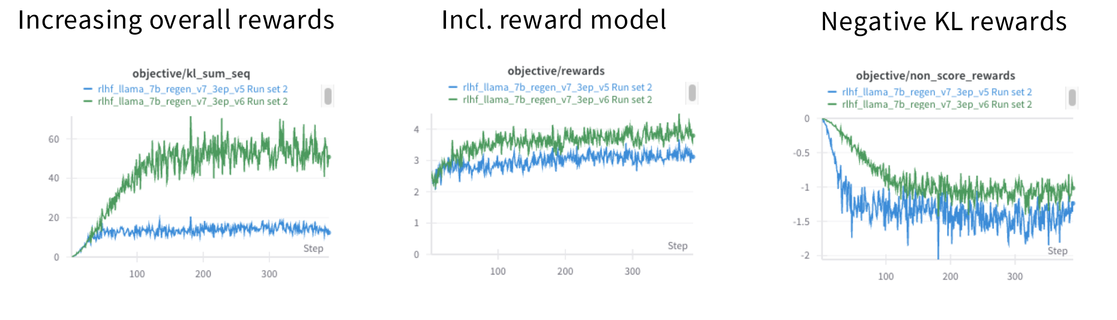
Figure 14.3 PPO training process curve

• Increasing overall rewards: Total reward rises. The name kl_sum_seq is somewhat misleading; it actually represents the sum of shaped rewards for each sequence. This "shaped reward" = task reward (e.g., high score for correct math answer) + KL penalty term (negative), measuring whether the model's overall performance is improving.
• Incl. reward model: Task reward rises. This metric measures the task reward the model directly obtains from the reward model, excluding the KL penalty. It reflects the model's performance on core tasks, such as the accuracy of answering questions and the ability to follow instructions.
• Negative KL rewards: Negative KL reward. This metric is the KL penalty term, i.e., the $-\beta \ast KL$ mentioned earlier. It shows that the model is indeed exploring and improving, but not out of control. This embodies the "proximal" idea of the PPO algorithm—allowing a certain degree of deviation, but limiting its magnitude.

These three curves together depict a healthy PPO training process: under the guidance of the reward model, the model gradually learns to generate better responses, while maintaining certain stability through the KL penalty, avoiding excessive deviation from the initial good behavior.

14.2.2 Why Do We Need Another RL Algorithm?

1. Why not directly use PPO?

PPO is currently one of the most successful online RL algorithms, widely used especially in LLM alignment. But it has two main drawbacks:

• Complicated implementation: PPO is not a simple "out-of-the-box" algorithm. It includes multiple complex components, such as: Rollout sampling, reward shaping, advantage estimation, loss calculation, etc. These steps require careful design and debugging, with a high threshold for novices or researchers pursuing rapid iteration.

• The burden of the Value Model: PPO needs an additional Value Model to estimate the value of states (V(s)), thereby computing the advantage function (A = Q - V).

  • Memory hungry: The value network shares the backbone structure with the policy network, but requires additional parameters and computational resources.
  • Additional tuning: The value network itself also needs training and optimization, increasing the complexity of the entire system and the hyperparameter search space. You need to simultaneously tune the policy network and the value network, ensuring they work together.

✅ Summary: Although PPO is powerful and effective, its engineering complexity is high, resource consumption is large, and tuning is difficult, especially in low-resource or efficiency-focused development scenarios, it appears cumbersome.

2. Why not directly use DPO?

DPO (Direct Preference Optimization) is a recent alternative that bypasses the traditional RL framework and directly optimizes from human preference data. But it also has the following limitations:

• Data not inherently pairwise: DPO's core idea is based on pairwise comparison data, i.e., given a prompt, there are two different responses (response A and response B), with annotation of which is better. However, in many practical application scenarios, the data we have is not naturally pairwise. For example, in the field of "verifiable rewards," the data is usually a single sequence plus an objective score (e.g., 1 for correct math answer, 0 for wrong). This scalar reward signal cannot be directly used for DPO.

• Offline algorithm: DPO is an offline algorithm. It performs one-time training on a fixed, pre-collected preference dataset. This is different from PPO's online learning nature. PPO can continuously generate new samples during training, obtain new feedback, and iteratively update the strategy accordingly. DPO "can theoretically be made online through iteration," but this increases complexity, losing its advantage as a simple offline method.

✅ Summary: DPO is very elegant and efficient in handling human preference data, but it is not suitable for non-pairwise, verifiable scalar reward scenarios, and its offline nature limits its application in tasks requiring continuous exploration and online learning.

14.2.3 GRPO: PPO with the Value Function Removed

GRPO (Group Relative Policy Optimization) is an algorithm proposed in the DeepSeekMath paper and brought to prominence in Deepseek-R1. GRPO, on the basis of PPO, removes the value function and advantage computation. This is the biggest change to PPO and the fundamental reason for its lightweight nature. And it adopts a completely new way to estimate "advantage"—namely "z-score within group."

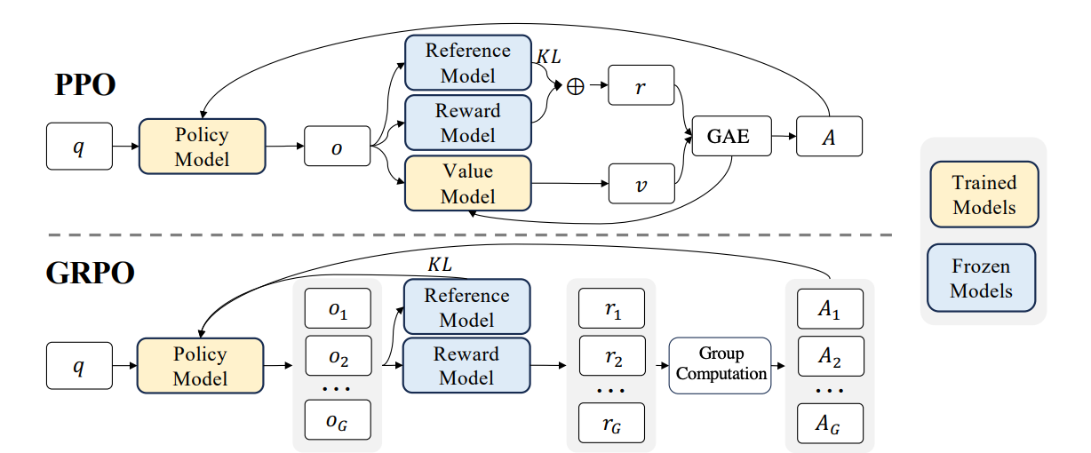
Figure 14.4 Comparison of PPO and GRPO

✅ In short, GRPO = PPO - Value Model + Group Z-Score Advantage.

GRPO's Objective Function

$${\mathcal{J}}_{GRPO}(\theta )=\mathbb{E}[q\sim P(Q),\{o_i{\}}_{i=1}^G\sim {\pi }_{{\theta }_{old}}(O|q)]\frac{1}{G}\sum _{i=1}^G(min(\frac{{\pi }_{\theta }(o_i|q)}{{\pi }_{{\theta }_{old}}(o_i|q)}{A}_i,\text{clip}(\frac{{\pi }_{\theta }(o_i|q)}{{\pi }_{{\theta }_{old}}(o_i|q)},1-ϵ,1+ϵ)A_i)-\beta {\mathbb{D}}_{KL}({\pi }_{\theta }||{\pi }_{ref}))$$

• The min(...) part: This is PPO's classic clipped objective function, used to update the policy ${\pi }_{\theta }$.
  • $\frac{{\pi }_{\theta }(o_i|q)}{{\pi }_{{\theta }_{old}}(o_i|q)}$ is the new-old policy probability ratio.
  • $A_i$ is the "advantage" of the $i$-th output $o_i$, which is GRPO's biggest innovation.
  • clip(...) is PPO's clipping mechanism, preventing policy updates from being too large.
• The $-\beta D_{KL}(...)$ part: This is the KL divergence penalty term, used to prevent the new policy ${\pi }_{\theta }$ from deviating too far from the reference policy ${\pi }_{ref}$, ensuring the stability of the generated results.
  • $\beta$ is the hyperparameter controlling the strength of the KL penalty.

PPO's objective function:

$$min(\frac{{\pi }_{\theta }(a|s)}{{\pi }_{{\theta }_k}(a|s)}{A}^{{\pi }_{{\theta }_k}}(s,a),\text{ clip}(\frac{{\pi }_{\theta }(a|s)}{{\pi }_{{\theta }_k}(a|s)},1-ϵ,1+ϵ)A^{{\pi }_{{\theta }_k}}(s,a))$$

The structure of GRPO and PPO objective functions is very similar, both containing probability ratios and clipping. The core difference lies in the source of A:

• PPO: A is computed through the value network V(s) and GAE, a complex and resource-intensive process.
• GRPO: A is computed through within-group z-score, a simple, fast process without additional models.

KL Divergence Calculation

$${\mathbb{D}}_{KL}({\pi }_{\theta }||{\pi }_{ref})=\frac{{\pi }_{ref}(o_i|q)}{{\pi }_{\theta }(o_i|q)}-\log \frac{{\pi }_{ref}(o_i|q)}{{\pi }_{\theta }(o_i|q)}-1$$

This is an approximate KL divergence formula. It is not in the standard integral form, but is approximated at each sampling point $o_i$. Its role is to measure the probability difference between the current policy ${\pi }_{\theta }$ and the reference policy ${\pi }_{ref}$ when generating a specific output $o_i$.

Within-Group z-score Advantage

$$A_i=\frac{r_i-\text{mean}(\{r_1,r_2,\cdots ,r_G\})}{\text{std}(\{r_1,r_2,\cdots ,r_G\})}$$

This is the soul of GRPO! It completely abandons the complex GAE calculation in PPO.

How to compute?

• For each question $q$, sample a group (G) of different responses $\{o_1,o_2,...,o_G\}$ from the old policy ${\pi }_{old}$.
• Use the reward model or verifiable rules to separately score these G responses, obtaining a group of rewards $\{r_1,r_2,...,r_G\}$.
• Calculate the mean and standard deviation of this group of rewards.
• Subtract the mean from each response $o_i$'s reward $r_i$, and divide by the standard deviation, to obtain its $A_i$.

Why is it called "z-score"?

In statistics, z-score represents how many standard deviations a data point is from the mean. Here, $A_i$ represents the "relative quality" of response $o_i$'s reward within the group. If $A_i>0$, it means this response is better than the group average; if $A_i<0$, it means it is worse than average.

Why is it effective?

• Simple and efficient: No need to train an additional value network, nor complex GAE calculations.
• Self-normalizing: Through within-group comparison, the problem of inconsistent reward scales between different questions is automatically eliminated. For example, one math problem might have a maximum of 10 points, while another might have a maximum of 5 points, but when compared within the same group, z-score can fairly reflect relative quality.
• Suitable for verifiable rewards: For a math problem, you can have the model generate multiple answers, then use a program to automatically determine whether each answer is correct (score 1 or 0), and then use z-score to distinguish which answer is "better."

In an online learning (sampling while updating) scenario, GRPO is essentially a policy gradient method using within-group normalized rewards.

💻 Code Interpretation: A Minimalist GRPO Implementation

The implementation of GRPO is very simple, without complex GAE calculations. Below we analyze the key code based on the GRPO algorithm implementation in the nano-aha-moment project. The following compute_pg_loss is a typical GRPO loss calculation function:

def compute_pg_loss(
    policy_model: Union[DeepSpeedEngine, PreTrainedModel], # Current language model to train
    batch: Dict[str, torch.Tensor], # A dictionary containing training data
    total_response_len: torch.Tensor, # Total number of valid tokens in the batch
    TEMPERATURE: float, # Temperature parameter during generation (affects log-prob calculation)
    KL_COEFFICIENT: float, # Hyperparameter controlling KL penalty strength
) -> Tuple[torch.Tensor, Dict[str, float]]:
    """
    Compute the policy gradient loss with KL penalty between policy and reference models.
    ...
    """
    # 1. Extract key tensors from batch
    input_ids = batch["input_ids"]  # [batch_size, seq_len], complete sequence (prompt + response)
    attention_mask = batch["attention_mask"]  # [batch_size, seq_len], indicates valid tokens
    labels = batch["labels"]  # [batch_size, seq_len], usually same as input_ids or shifted right by one
    labels_mask = batch["labels_mask"]  # [batch_size, seq_len], 1 indicates response token, 0 indicates prompt or padding
    advantages = batch["advantages"]  # [batch_size, seq_len], "advantage" value for each token (from within-group normalization)
    ref_logps = batch["ref_log_probs"]  # [batch_size, seq_len-1], log-prob of reference model on response tokens (length is one less than input_ids)

    # 2. Build model inputs
    model_inputs = {
        "input_ids": input_ids,
        "attention_mask": attention_mask,
        "labels": labels,
        "labels_mask": labels_mask,
    }

    # 3. Calculate token log-probabilities of current policy
    logps = compute_token_log_probs(policy_model, model_inputs, TEMPERATURE)  # Forward pass policy_model on input_ids, get log-probability of each token, output shape [batch_size, seq_len-1] because the model predicts input_ids[1:]

    # 4. Align mask and compute KL penalty term
    labels_mask = labels_mask[..., 1:].to(logps.dtype)  # Also right-shift labels_mask by one, align with logps, only keep response token mask, output shape [batch_size, seq_len-1]
    
    # Direct KL calculation requires summing over the entire vocabulary (sum(p * log(p/q))), which is computationally expensive. We use an approximation of Bregman divergence, and this approximation only depends on logps and ref_logps (i.e., token-level log-prob), which is very efficient.
    ref_logratio = ref_logps - logps
    kl_penalty = torch.exp(ref_logratio) - 1 - ref_logratio  # [batch_size, seq_len-1]
    kl_penalty = kl_penalty * labels_mask  # [batch_size, seq_len-1], only compute KL penalty for response tokens, ignore prompts

    # 5. Calculate auxiliary statistics (not involved in gradient)
    with torch.no_grad():
        entropy = -logps.sum() / labels_mask.sum()  # scalar
        zero_advantages = close_to_zero(advantages[..., 1:], labels_mask)  # scalar

    # 6. Calculate policy gradient loss
    policy_loss = -logps * advantages[..., 1:]  # [batch_size, seq_len-1], advantages[..., 1:] takes advantage from the 2nd token, aligned with logps
    policy_loss = policy_loss * labels_mask  # [batch_size, seq_len-1]

    # 7. Combine total loss and normalize
    loss = (policy_loss + KL_COEFFICIENT * kl_penalty).sum() / total_response_len  # Weighted sum of policy loss and KL penalty, divide by total_response_len, normalize total loss to average loss per valid token, making loss values comparable across different batch sizes.

    # 8. Build returned metrics dictionary
    metrics = {
        "policy_loss": policy_loss.sum().item() / total_response_len.item(),
        "kl_penalty": kl_penalty.sum().item() / total_response_len.item(),
        "entropy": entropy.item() / total_response_len.item(),
        "zero_advantages_ratio": zero_advantages.item() / total_response_len.item(),
    }

    return loss, metrics

In GRPO, the advantage computation is extremely simple; its core is "within-group z-score normalization," and for numerical stability, a small constant of 1e-4 is added. Below is its implementation code:

# 1. Data validation and grouping

assert len(all_generations) == len(all_finish_reasons) # all_generations is all model-generated responses, all_finish_reasons is the end reason for each response (e.g., "stop" or "length"), samples is the original input samples
assert len(all_generations) == len(samples) * GENERATIONS_PER_SAMPLE # GENERATIONS_PER_SAMPLE is a hyperparameter indicating how many different responses to generate for each input sample (e.g., 3). So total responses = number of samples × number of generations per sample.

# Group all generated responses by sample. For example, if GENERATIONS_PER_SAMPLE=3, then groups = [[0,1,2], [3,4,5], ...], where [0,1,2] corresponds to the three responses generated for the first sample
groups = [
    list(range(i, i + GENERATIONS_PER_SAMPLE)) for i in range(0, len(all_generations), GENERATIONS_PER_SAMPLE)
]

# 2. Initialize storage variables

all_query_token_ids, all_responses_token_ids, all_samples, all_rewards = [], [], [], []
stats = { "response_lengths": [], "rewards": [], "non_stop_rate": [], }

# 3. Core loop: process each sample and its generated response group
# For current sample sample, get its corresponding group_indices (e.g., [0,1,2]), then extract the group's end reason, token ID, and decoded text
for sample, group_indices in zip(samples, groups):
    finish_reasons = [all_finish_reasons[i] for i in group_indices]
    response_token_ids = [all_generations[i] for i in group_indices]
    responses = tokenizer.batch_decode(response_token_ids, skip_special_tokens=False)

    # For each response resp in the group, call compute_reward function to calculate its reward score. compute_reward is your custom function, e.g., to determine if a math problem is answered correctly, whether code can run, etc.
    rewards_and_metrics = [compute_reward(resp, sample, EOS_TOKEN) for resp in responses]
    rewards, reward_metrics = zip(*rewards_and_metrics) # zip(*rewards_and_metrics) unpacks (reward, metrics) tuples into two lists: rewards and reward_metrics

    # 4. Key step: compute within-group normalized "advantage" (Advantages)
    rewards = np.array(rewards)
    advantages = (rewards - rewards.mean()) / (rewards.std() + 1e-4) # rewards - rewards.mean(): calculate the deviation of each response's reward relative to the group mean; divide by group standard deviation to get z-score; when all rewards in the group are the same (standard deviation is 0), direct division by 0 causes NaN errors. Adding a tiny constant of 1e-4 can avoid this situation, ensuring computational stability

    # Expand each response's scalar advantage value resp_adv to a sequence of the same length as the response's tokens, so that the advantage signal can be aligned with each token's log-probability, thus computing the policy gradient loss
    per_token_advantages = [[adv] * len(resp) for adv, resp in zip(advantages, response_token_ids)]

    # 5. Collect final data and return
    # Append current group's data (rewards, samples, token IDs) to global lists for subsequent unified processing
    all_query_token_ids.extend([sample["input_ids"]] * GENERATIONS_PER_SAMPLE)
    all_responses_token_ids.extend(response_token_ids)
    all_advantages.extend(per_token_advantages)

    # Record some useful statistics, such as average reward, proportion of abnormal endings, response length, etc.
    stats["rewards"].extend(rewards)
    stats["non_stop_rate"].extend([fr != "stop" for fr in finish_reasons])
    stats["response_lengths"].extend([len(ids) for ids in response_token_ids])

    for rm in reward_metrics:
        for k, v in rm.items():
            stats.setdefault(f"reward_metrics/{k}", []).append(v)

# Package all data into a dictionary episodes for use by the subsequent compute_pg_loss function
episodes = {
        "all_query_token_ids": all_query_token_ids,
        "all_response_token_ids": all_responses_token_ids,
        "all_advantages": all_advantages,
    }

    return episodes, stats

GRPO's Actual Effects

How does GRPO actually perform? The figure below shows model performance on two mathematical reasoning benchmarks:

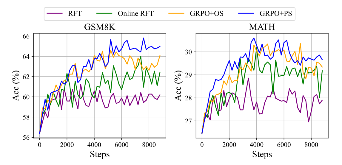
Figure 14.5 Performance comparison of GRPO with other training methods on two mathematical reasoning benchmarks

The left figure GSM8K is an elementary school math word problem dataset, and the right figure MATH is a more difficult high school math competition problem dataset. The Y-axis is accuracy (Acc %), and the X-axis is training steps. There are multiple curves in the figure, representing different training methods:

• RFT (Reinforcing Fine-Tuning): This is the most basic method. It only rewards "correct answers," without considering the generation process. It can be understood as "as long as the result is correct, regardless of the process." Represented by a purple line in the figure.
• Online RFT: This is the online version of RFT, possibly meaning it dynamically samples and updates during training, rather than using a fixed dataset. Represented by a green line in the figure.
• GRPO+OS (Group Relative Policy Optimization + Online Sampling): This is the standard GRPO method, i.e., the "within-group z-score normalization" advantage calculation we discussed earlier. Represented by an orange line in the figure.
• GRPO+PS (Group Relative Policy Optimization + Process Supervision): This adds "process supervision" on top of GRPO. This means not only the final answer is rewarded, but also the correct problem-solving steps are rewarded. Represented by a blue line in the figure.

From both figures, we can draw the following conclusions:

• GRPO significantly outperforms RFT: Whether on GSM8K or MATH, the orange line (GRPO+OS) and the blue line (GRPO+PS) are both significantly higher than the purple line (RFT). This shows that the GRPO algorithm itself is effective, and it can help the model learn better strategies, thereby achieving higher accuracy.
• Process supervision (PS) brings additional gains: At most training steps, the blue line (GRPO+PS) is slightly higher than the orange line (GRPO+OS). This shows that if supervision signals about the "problem-solving process" can be provided, the model's performance can be further improved.
• GRPO's stability: Compared to the more volatile RFT and Online RFT curves, GRPO's curve is relatively smoother, reflecting the stability of its algorithm design.

14.2.4 GRPO's Potential Flaw: Length Bias

Although GRPO is highly effective, the academic community (such as the "Dr. GRPO" paper) points out that it has mathematical flaws:

1. Biased Gradient

GRPO normalizes rewards or computes advantages through "within-group z-score," which is done to improve training stability without introducing a value function. However, the standard deviation (stdev) involved in computing this z-score may depend on the observed samples (possibly related to the output of the current policy), making the entire process no longer a strict unbiased baseline subtraction, which may introduce slight bias in theory.

What does an unbiased gradient version of GRPO look like?

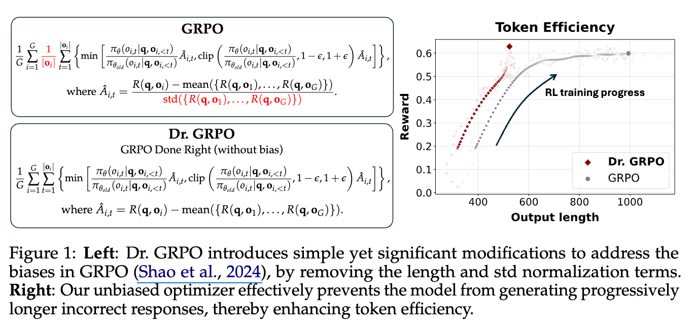
Figure 14.6 Mathematical formula and performance comparison of Dr. GRPO and standard GRPO

Dr. GRPO's core change is the removal of $\frac{1}{|o_i|}$ (response length normalization) and $\frac{1}{\text{std}(\{R(q,o_1),\dots ,R(q,o_G)\})}$ (standard deviation normalization) in the original GRPO, thereby correcting the response length bias and problem difficulty bias in GRPO.

The right figure shows the relationship between reward and output length during training for GRPO and Dr. GRPO. By removing the bias, Dr. GRPO effectively prevents the model from generating unnecessarily verbose responses (especially when answering incorrectly), thereby improving token efficiency.

2. Length Bias

The standard deviation is used to "upweight" those "too easy" or "too hard" questions.

This bias stems from the fact that in the GRPO (Group Relative Policy Optimization) objective function, the advantage function is divided by the response length $|o_i|$.

In the GRPO objective function, the gradient update portion for a single response $o_i$ at time step $t$ involves the following term: [ \dots \times \frac{\hat{A}_{i,t}}{|o_i|} \dots ] Where:

• $|o_i|$: represents the length of response $o_i$ (number of tokens).
• ${\hat{A}}_{i,t}$: is the advantage function, calculated as ${\hat{A}}_{i,t}=R(q,o_i)-\text{mean}(\{R(q,o_1),\dots ,R(q,o_G)\})/\text{std}(\{R(q,o_1),\dots ,R(q,o_G)\})$, where $R(q,o_i)$ is the return of response $o_i$.

Impact on correct answers (positive advantage): When the advantage function ${\hat{A}}_{i,t}$ is positive (${\hat{A}}_{i,t}>0$, indicating a correct answer), dividing ${\hat{A}}_{i,t}$ by a smaller response length $|o_i|$ yields a larger value. This means the model receives a larger gradient update, thereby incentivizing the model to tend to generate shorter correct answers, i.e., preferring conciseness. Impact on incorrect answers (negative advantage): When the advantage function ${\hat{A}}_{i,t}$ is negative (${\hat{A}}_{i,t}<0$, indicating an incorrect answer), dividing ${\hat{A}}_{i,t}$ by a larger response length $|o_i|$ yields a relatively smaller (i.e., less negative) penalty. This means the model will lessen the penalty for longer incorrect answers.

This mechanism causes the model to tend to generate longer responses when generating incorrect answers, a "the more wrong, the longer" phenomenon.

14.3 Case Studies

Here we introduce three works on RLVR:

• Deepseek R1: The core of many recent RLVR works, containing many interesting details.
• Kimi K1.5: Concurrent with R1, RLVR provides complementary details to R1.
• Qwen 3: The latest open-source reasoning model attempt, low-data RLVR

14.3.1 DeepSeek R1

The DeepSeek R1 paper caused quite a sensation.

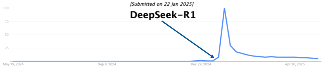
Figure 14.7 DeepSeek-R1 attracts widespread attention

What's special about R1?

• Performance surpasses OpenAI O1
• Open RL recipe (and quite simple)
  • Ended speculation about the necessity of MCTS/PRM
• SFT insights (including R1-zero and distil-r1)

They follow the GRPO results from the DeepSeekMath paper.

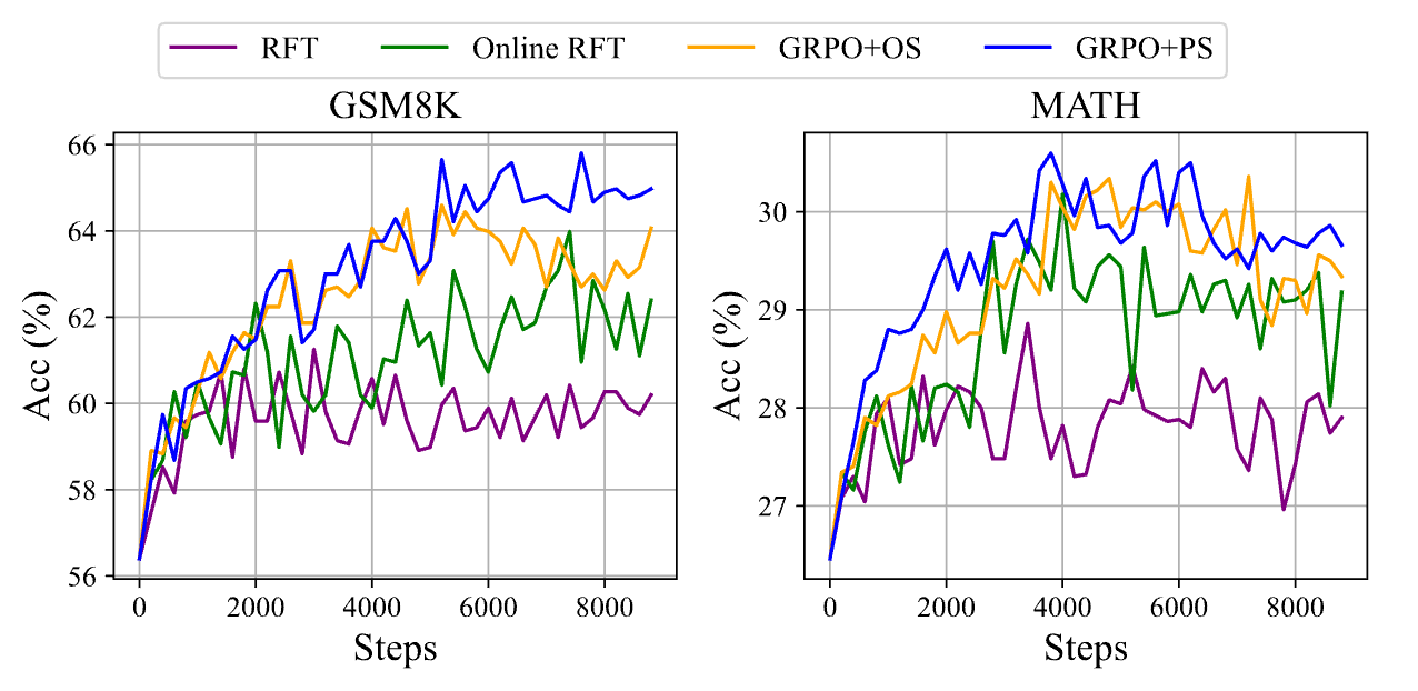
Figure 14.8 Comparison of GRPO and other algorithms

The figure shows the changes in accuracy (Acc %) with training steps (Steps) for four different algorithms (RFT, Online RFT, GRPO+OS, GRPO+PS) on two datasets—GSM8K (left) and MATH (right)—during the training process.

The success of DeepSeek R1 proves the huge potential of pure reinforcement learning on reasoning tasks.

R1-Zero: Pure RL

• Setup: Run GRPO directly on the Base model (DeepSeek-V3).
• Reward:
  • Accuracy reward: Is the answer correct? (via rule matching or compiler validation).
  • Format reward: Force the model to wrap its thinking process with <think> and </think> tags.
  • Data: Not disclosed

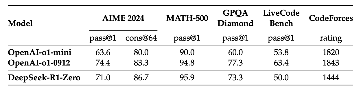
Figure 14.9 Performance comparison of Deepseek-R1-Zero and OpenAI-o1 on related reasoning benchmarks

In most cases, DeepSeek-R1 performs comparably to or better than o1-mini, and on several tasks it is comparable to o1-0912. However, in the code domain, DeepSeek-R1's performance is not as good as o1 model.

Deepseek-R1-Zero produced an interesting phenomenon called Aha Moment (顿悟时刻): In the middle of training, the model began to learn self-reflection (Self-correction), such as "wait, I calculated it wrong, I should try again...".

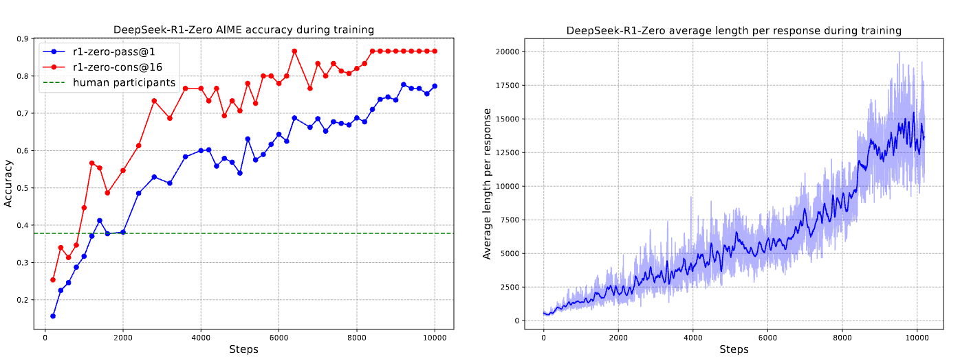
Figure 14.10 DeepSeek-R1-Zero's AIME accuracy and average response length on the training set during training

The increase in thinking time promotes the autonomous development of complex behaviors. Specifically, DeepSeek-R1-Zero increasingly exhibits advanced reasoning strategies, such as reflective reasoning and systematic exploration of alternative solutions, significantly improving its performance on verifiable tasks like math and coding.

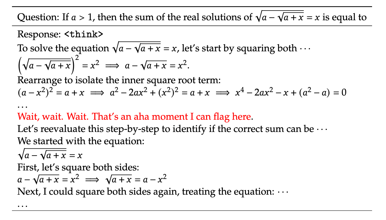
Figure 14.11 Discovery of aha moment

Notably, during the training process, DeepSeek-R1-Zero exhibits an "aha moment," characterized by a sudden increase in the frequency of using the word "wait" during reflection. This moment marks a significant change in reasoning patterns, and clearly demonstrates the self-evolution process of DeepSeek-R1-Zero.

But maybe a bit overstated?

GRPO uses a biased optimization objective. When the optimization objective (whether the reward model or DPO's loss function) is inadvertently biased toward outputs of a specific length, the model, in the process of pursuing the maximization of this objective, will exhibit a "length bias."

Figure 14.6 Mathematical formula and performance comparison of Dr. GRPO and standard GRPO

The base model had already exhibited the "aha moment" phenomenon:

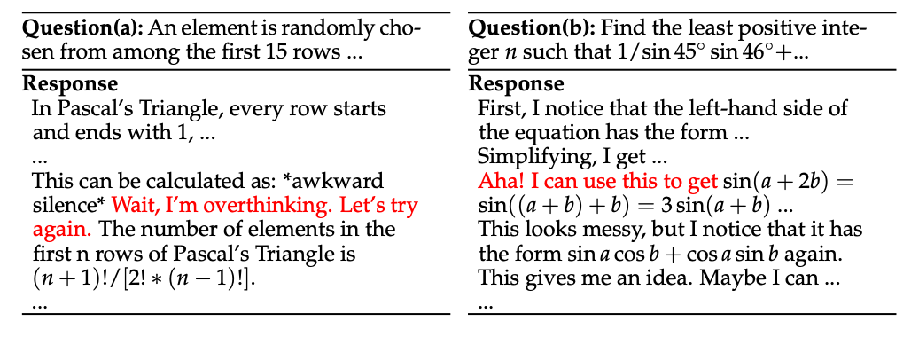
Figure 14.12 Case where DeepSeek-V3-Base had already exhibited the aha-moment phenomenon

DeepSeek-R1

Although DeepSeek-R1-Zero exhibits powerful reasoning capabilities, it also faces some problems. DeepSeek-R1-Zero has challenges in readability and language mixing, because DeepSeek-V3-Base is trained on multiple languages, especially English and Chinese. To address these issues, the Deepseek team developed DeepSeek-R1, whose process is shown in Figure 2.

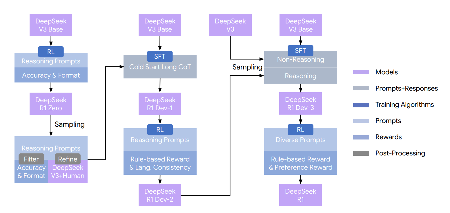
Figure 14.13 Deepseek-R1 development process

Stage 1: DeepSeek-R1-Zero

Using DeepSeek-V3-Base as the base model, completely relying on reinforcement learning, the reward signal mainly comes from rule-based rewards, including accuracy and format rewards.

Stage 2: Data Collection

Using DeepSeek-V3-Base as the base model, using cold-start long chain-of-thought data for SFT training to obtain DeepSeek-R1-Dev1.

For the collection of cold-start long chain-of-thought data, specifically, they first collected thousands of high-quality, diverse reasoning prompts. For each prompt, DeepSeek-R1-Zero was used to generate multiple reasoning trajectories at a relatively high temperature of 1.0. Next, these generated contents were filtered to retain only those with correct final answers and readable formats. For math output, they used sympy(https://www.sympy.org/) for parsing and expression comparison; for formatting, they applied rules such as duplicate detection and language mixing filtering. Finally, DeepSeek-V3 was prompted to refine the reasoning and summary to ensure correct format and human-friendly expression. In particular, to address the language mixing issue, they instructed DeepSeek-V3: "Translate the thinking process to the same language as the question." Since DeepSeek-R1-Zero's summary only provides the final answer, they used the summary prompt in Listing 1 to generate a concise, human-readable solution that outlines the reasoning steps and final results.

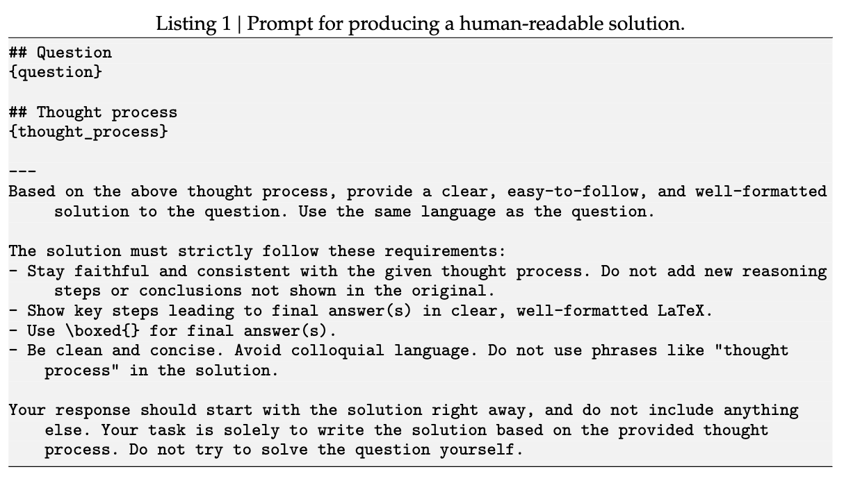
Figure 14.14 Prompt for generating human-readable answers

On the basis of DeepSeek-R1-Dev1, the reward signal uses rule-based rewards (accuracy + format) and language consistency rewards, and RL training is performed to obtain DeepSeek-R1-Dev2.

Stage 3: Post-training

Using DeepSeek-V3-Base as the base model, using 800k (600k reasoning-related data + 200k non-reasoning data) supervised data for SFT training to obtain DeepSeek-R1-Dev3.

Reasoning trajectories are generated by rejection sampling from the DeepSeek-R1-Dev2 checkpoint, and approximately 600k reasoning-related training samples are collected.

For non-reasoning data, such as writing, factual QA, self-recognition, and translation, the DeepSeek-V3 pipeline is used and part of the SFT dataset of DeepSeek-V3 is reused. Software engineering-related data, including program repair and front-end web development, is also integrated to enhance the model's ability to solve real-world problems. For some non-reasoning tasks, before prompting to answer questions, DeepSeek-V3 is called to generate potential chain-of-thought. However, for simpler queries, such as "hello," we do not provide CoT as a response. Finally, we collected about 200k training samples unrelated to reasoning.

On DeepSeek-R1-Dev3, RL is continued. For reasoning data, rule-based rewards are used; for general data, since there is no explicit rule-based reward signal for right and wrong, Reward Models are used to capture human preferences in complex and nuanced scenarios, calculating rewards from both helpful and safety perspectives.

How does DeepSeek-R1 perform?

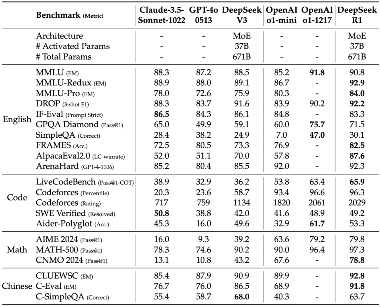
Figure 14.15 Comparison of DeepSeek-R1 and other models

Distillation: Can we convert a non-reasoning model into a reasoning model?

Another huge contribution of R1 is proving that the reasoning ability of a large model can be distilled into a small model. Using the 800k pieces of data generated by R1 to fine-tune Qwen2.5, let the student model (Qwen2.5) learn the reasoning ability of the teacher model (R1)!

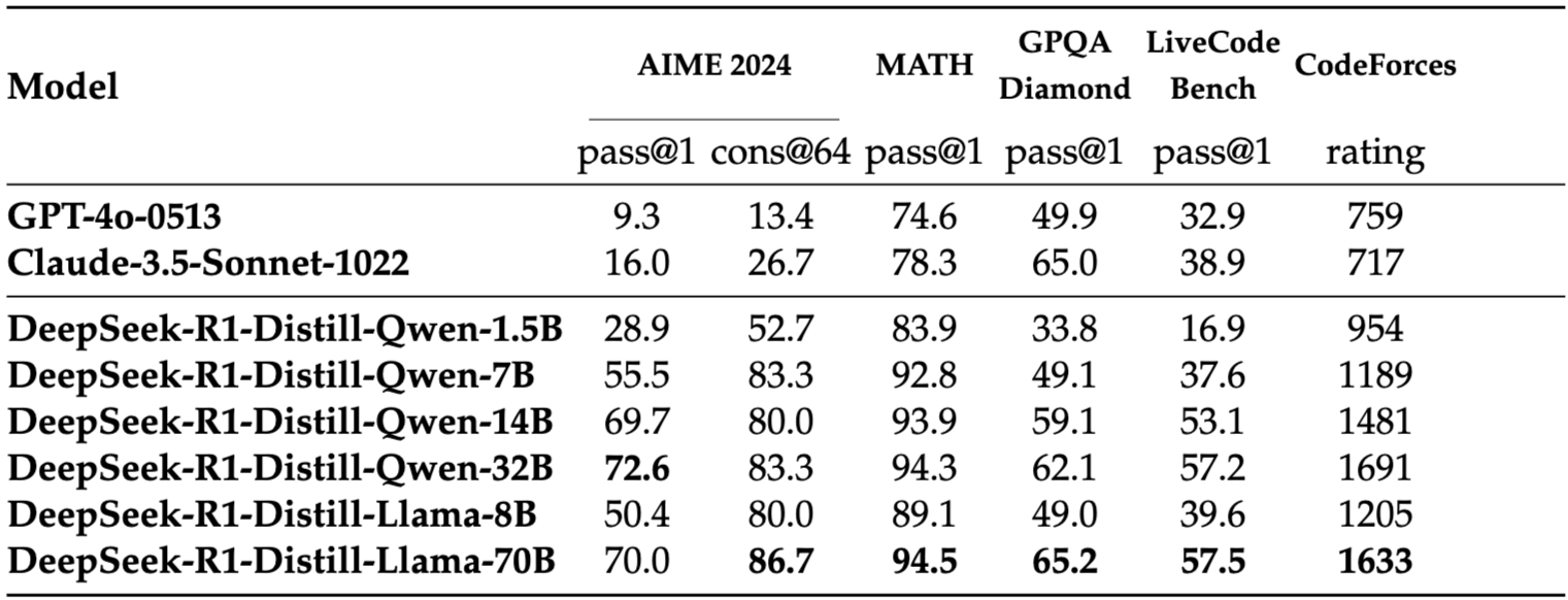
Figure 14.16 Comparison of Deepseek-R1 distilled models and other models

Using a Small Number of High-Quality SFT Samples to Improve Math Reasoning

In addition to the Deepseek-R1 paradigm that can yield a powerful reasoning model, we can also obtain a reasoning model with decent performance by directly using Base+SFT.

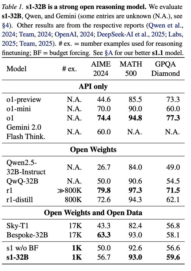
Figure 14.17 s1 uses 1k high-quality samples to improve math reasoning ability

The Li Fei-Fei team's article s1: Simple test-time scaling uses 1k high-quality data with long chain-of-thought, and performs SFT on Qwen2.5-32B-Instruct to obtain strong math reasoning ability.

Shanghai Jiao Tong University's Liu Pengfei team also reached a similar conclusion in LIMO: Less is More for Reasoning, using 800 high-quality data with long chain-of-thought, and performing SFT on Qwen2.5-32B-Instruct greatly improved the model's math reasoning ability.

Figure 14.18 s1 uses 1k high-quality samples to improve math reasoning ability

However, it should be noted that using a small number of samples to improve model reasoning ability requires a high capability of the base model. The above results work well on Qwen2.5-32B-Instruct, but work poorly on Qwen2.5-7B-Instruct and Qwen2.5-3B-Instruct.

Using a Small Number of High-Quality Samples for RL to Improve Math Reasoning

Reasoning models can also be obtained through the Base+RL route. In addition to Deepseek-R1-Zero, two works LIMR (Qwen2.5-Math-7B+PPO) and Less is More: Improving LLM Alignment via Preference Data Selection (llama3-8B+DPO) also prove the feasibility of this route.

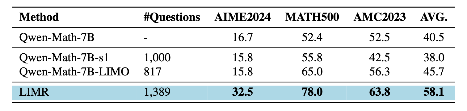
Figure 14.19 Performance comparison of limr and other models

Unsuccessful Attempts

The Deepseek-R1 team also shared some unsuccessful attempts they made in the early stages of DeepSeek-R1 development:

Process Reward Model (PRM): PRM attempts to rerank, guide search, or improve thinking by evaluating intermediate reasoning steps, but has several problems in practical applications.

• Difficult to clearly define fine-grained intermediate steps. It's hard to give a general, automatically evaluable definition of "correct intermediate steps," leading to difficulties in stepwise annotation and evaluation of intermediate processes.
• The challenge of judging whether a current intermediate step is correct. Automatically annotating the correctness of an intermediate step is often unreliable, and manual annotation is difficult to scale, making it hard to land in large-scale training.
• After introducing the model, reward hacking behavior is easy to produce, and the cost is high. Once a model-based reward is introduced, the model may find cheating paths to increase rewards, thus deviating from the true goal; in addition, retraining the reward model requires additional computing power and data, increasing the complexity and cost of the training pipeline.

Monte Carlo Tree Search (MCTS): Inspired by AlphaGo and AlphaZero, they explored using Monte Carlo tree search (MCTS) to enhance the scalability of test-time computation. This method involves breaking the answer into smaller parts to allow the model to systematically explore the solution space. To achieve this, the model is prompted to generate multiple labels, which correspond to the specific reasoning steps required for the search.

• Unlike chess, where the search space is relatively clear, token generation presents an exponentially larger search space. To solve this problem, they set a maximum expansion limit for each node, but this may cause the model to fall into local optima.
• Second, the value model directly affects the generation quality because it guides every step of the search process. Training a fine-grained value model is itself very difficult, which makes it difficult for the model to iteratively improve. Although the core success of AlphaGo depends on training a value model to gradually improve its performance, due to the complexity of token generation, this principle is difficult to replicate in our current setup.

In summary, although MCTS can improve performance during inference when paired with a pre-trained value model, iteratively improving model performance through self-search remains a significant challenge.

14.3.2 Kimi k1.5

Long Chain-of-Thought Reasoning Strategy

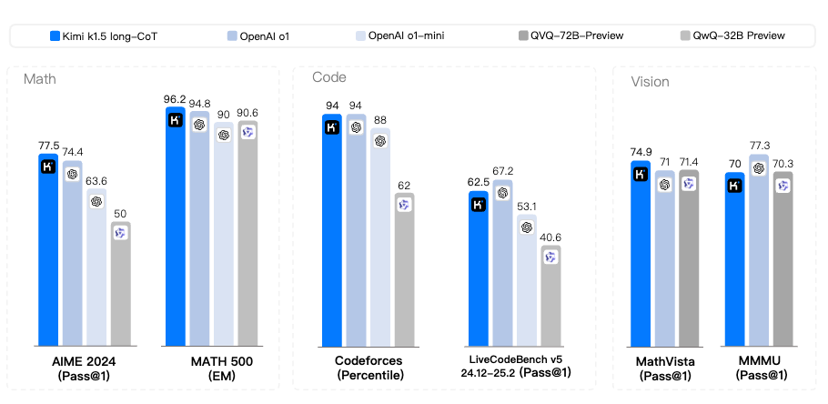
Figure 14.20 Kimi-k1.5 long chain-of-thought results

Key steps:

• Data construction (difficulty filtering)
• Long-CoT SFT
• RL (using their own policy gradient loss)

Data Management

The quality and diversity of the RL Prompt Set plays a key role in ensuring the effectiveness of reinforcement learning. A carefully constructed prompt set can not only guide the model for robust reasoning, but also mitigate the risk of reward hacking and overfitting to surface patterns. Specifically, three key attributes define a high-quality RL prompt set:

• Diverse coverage: Prompts should cover a wide range of disciplines, such as STEM, coding, and general reasoning, to enhance the model's adaptability and ensure broad applicability across different fields. The kimi team developed a labeling system to classify prompts by domain and discipline, ensuring balanced representation across different disciplines
• Balanced difficulty: The prompt set should contain a good distribution range of questions of varying difficulty, such as easy, medium, and hard, to facilitate progressive learning and prevent overfitting to a specific level of complexity. A model-based method is adopted, which leverages the model's own capabilities to adaptively evaluate the difficulty of each prompt. By leveraging this method, most very simple samples can be pre-filtered, and different sampling strategies can be easily explored during RL training.
• Precise evaluability: Prompts should allow verifiers to perform objective and reliable evaluation, ensuring model properties. To avoid potential reward hacking, it is necessary to ensure that the reasoning process and final answer for each prompt can be accurately verified. Empirical observations show that some complex reasoning problems may have relatively simple and easily guessed answers, which can lead to false positive verifications—i.e., the model arrives at the correct answer through an incorrect reasoning process. To address this problem, they excluded questions prone to such errors, such as multiple choice, true/false, and proof questions. In addition, for general Q&A tasks, we propose a simple but effective method to identify and remove prompts that are easy to hack. Specifically, we prompt the model to guess potential answers without any CoT reasoning steps. If the model predicts the correct answer within N attempts, the prompt is considered too easy to hack and is removed. They found that setting N = 8 can remove most prompts that are easy to hack.

Long Chain-of-Thought (Long-CoT) SFT

Before the model enters the complex reinforcement learning stage, supervised fine-tuning is used to let the model initially learn and internalize a set of high-quality, human-like complex reasoning capabilities. This is like "warming up" the model, ensuring that it can better understand and utilize reward signals in subsequent RL training to generate valuable reasoning processes.

Select questions from the refined RL prompt set. Using "prompt engineering" techniques, construct a small but high-quality "long CoT reasoning path" for these questions. These paths contain precisely verified reasoning steps, applicable to text and image inputs. Similar to rejection sampling (RS), but the focus is on using carefully designed prompts to "guide" the model to generate long CoT reasoning paths, rather than simply selecting the best results from a large number of random generations. Through the above steps, we have constructed a dataset for SFT.

Kimi RL

We hope to maximize the model's expected reward on the reference answer, without making the model deviate too much from the original behavior. The objective function is:

$$\underset{\theta }{max}{\mathbb{E}}_{(x,y^{\ast })\sim \mathcal{D}}[{\mathbb{E}}_{(y,z)\sim {\pi }_{\theta }}[r(x,y,y^{\ast })]-\tau \text{KL}({\pi }_{\theta }(x)||{\pi }_{{\theta }_i}(x))]$$

Borrowing from DPO's idea of reward-free preference optimization, instead of directly designing a reward function, it indirectly defines a "pseudo-reward" by comparing the difference between the current policy and the reference policy, and then uses a squared loss to approximate it.

Here we assume the existence of an "ideal policy" ${\pi }^{\ast }$ (which can be understood as a human preference distribution or expert strategy), and then through DPO's idea, link the reward function $r$ with the policy ratio. Specifically, the reward minus a normalization constant $\tau \log Z$ is equal to $\tau$ times the log ratio of the ideal policy to the reference policy. This derivation is based on the "non-parametric assumption," meaning that the reward function is not explicitly modeled, but is implicitly determined by policy differences (similar to the core idea of DPO). The final goal is to "solve for $r$," i.e., express the reward function as a function of the policy.

$r(x,y,y^{\ast })-\tau \log Z=\tau \log \frac{{\pi }^{\ast }(y,z|x)}{{\pi }_{{\theta }_i}(y,z|x)}$

Because directly optimizing the original objective can be difficult, a squared error loss is used here for approximate optimization. Its goal is to make the output of the current policy ${\pi }_{\theta }$ as close as possible to the reward expression corresponding to the "ideal policy ${\pi }^{\ast }$." Note that sampling here is from the reference policy ${\pi }_{{\theta }_i}$, not the current policy ${\pi }_{\theta }$—this is to stabilize training and avoid bias from bootstrapping. The final loss $L(\theta )$ is the squared error after taking expectations over all samples and sampling results.

$L(\theta )={\mathbb{E}}_{(x,y^{\ast })\sim \mathcal{D}}\left[{\mathbb{E}}_{(y,z)\sim {\pi }_{{\theta }_i}}\left[{(r(x,y,y^{\ast })-\tau \log Z-\tau \log \frac{{\pi }_{\theta }(y,z|x)}{{\pi }_{{\theta }_i}(y,z|x)})}^2\right)\right]$

The final regularized baseline policy gradient for updating model parameters $\theta$:

$$\frac{1}{k}\sum _{j=1}^k({\mathrm{\nabla }}_{\theta }\log {\pi }_{\theta }(y_j,z_j|x)(r(x,y_j,y^{\ast })-\overline{r})-\frac{\tau }{2}{\mathrm{\nabla }}_{\theta }{(\log \frac{{\pi }_{\theta }(y_j,z_j|x)}{{\pi }_{{\theta }_i}(y_j,z_j|x)})}^2)$$

For each sampled $(y_j,z_j)$, calculate its gradient contribution. The gradient consists of two parts: 1. Reward-driven policy improvement; 2. Regularization-driven behavior constraint. Finally, take the average ($\frac{1}{k}\sum$) to get the final update direction.

Length Control

The Kimi team observed an "overthinking" phenomenon, i.e., the length of model responses increased significantly during RL training. Although this brings better performance, overly long reasoning processes are costly during training and inference, and overthinking is generally not preferred by humans. To address this, they introduced a length reward to curb the rapid growth of token length, thereby improving the model's token efficiency.

[ \text{len_reward}(i) = \begin{cases} \lambda & \text{If } r(x, y_i, y^) = 1 \ \min(0, \lambda) & \text{If } r(x, y_i, y^) = 0 \end{cases}\text{, where } \lambda = 0.5 - \frac{\text{len}(i) - \text{min_len}}{\text{max_len} - \text{min_len}}. ]

This length penalty mechanism encourages the model to generate concise responses while giving correct answers. For incorrect answers, it never gives any positive length reward, and imposes additional penalties on overly long incorrect answers.

Additional Details

Sampling strategy:

• Assign difficulty labels to the dataset, from easy to hard
• The sampling proportion of questions is proportional to (1-success_rate) to avoid repeating already solved problems

Rewards:

• For code—use problems with ground truth solutions to generate new test cases
• For math—use 800k samples to train a CoT reward model for answer equivalence checking

Scaling Results

Kimi-k1.5 is roughly comparable in performance to "o1", and may even be better:

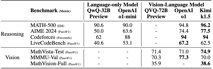
Figure 14.21 Kimi-k1.5 long chain-of-thought results

Other interesting results:

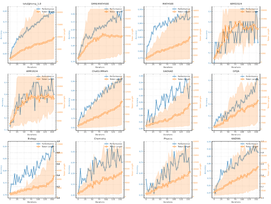
Figure 14.22 Kimi-k1.5 long chain-of-thought results

Ablation Experiments

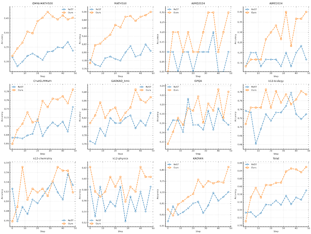
Figure 14.23 Comparison of Kimi-k1.5 and ReST for policy gradient optimization

Note that the above scores come from an internal long-cot model with a much smaller size than the k1.5 long-CoT model

14.3.3 Qwen 3: Thinking Mode Fusion

The largest model in the Qwen3 family, Qwen3-235B-A22B, outperforms OpenAI-o1 and Deepseek-R1, and even Qwen3-32B is comparable to o1.

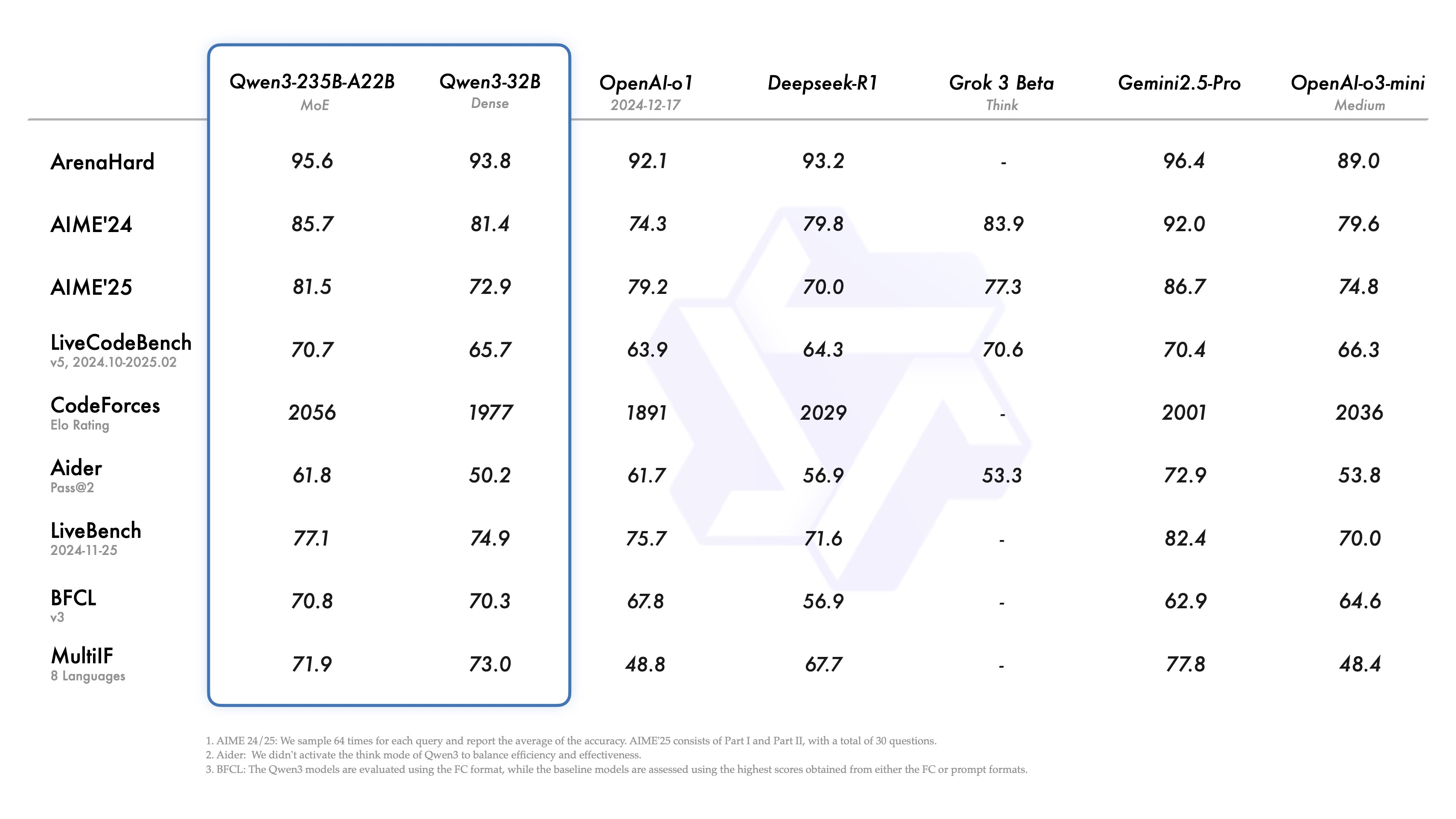
Figure 14.24 Performance comparison of Qwen3 and other models

The Qwen3 post-training process is carefully designed with two core objectives:

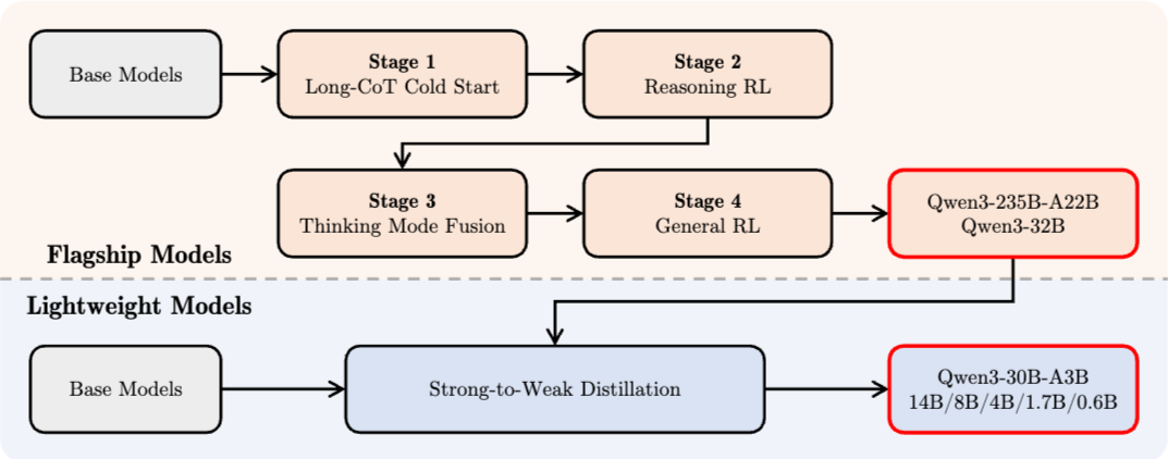
Figure 14.25 Post-training pipeline of Qwen3 series models

• Thinking control: This involves the integration of two different modes, i.e., "non-thinking" mode and "thinking" mode, allowing users to flexibly choose whether the model reasons, and to control the depth of thinking by specifying the token budget of the thinking process
• Strong-to-weak distillation: This aims to simplify and optimize the post-training process for lightweight models. By leveraging the knowledge of large models, the computational cost and development effort required to build small models are greatly reduced.

SFT + Reasoning Reinforcement Learning

We all know this routine now, and Qwen also uses a lot of it.

• Filter by difficulty (via best-of-n, e.g., kimi)
  • Remove questions the model can answer correctly without CoT
  • Remove content too similar to validation data
• Manually filter the quality of CoT (guessing vs. correct answer)
• Use GRPO for RL on only 3995 examples

Qwen 3 Specific New Content

Thinking mode fusion—control the length of CoT.

1. Mix labeled non-thinking and thinking data

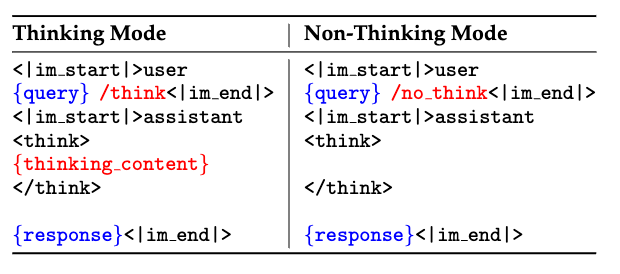
Figure 14.26 Example of SFT data in the thinking mode fusion stage

2. Early stopping through special strings

An additional advantage of thinking mode fusion is that once the model learns to respond in both non-thinking and thinking modes, it naturally develops the ability to handle intermediate cases—generating responses based on incomplete thinking. This capability lays the foundation for budget control over the model's thinking process. Specifically, when the model's thinking length reaches a user-defined threshold, we manually stop the thinking process and insert a stop thinking instruction: "Considering the user's limited time, I must directly provide a solution based on the thinking. \n</think>.\n\n". After inserting this instruction, the model will generate the final response based on the reasoning accumulated so far. Notably, this capability is not explicitly trained, but emerges naturally through the application of thinking mode fusion.

Test Time Scaling (TTS)

This figure shows how model performance (Pass@1) varies with "thinking budget" (in K tokens) in two modes ("thinking mode" and "non-thinking mode") on different benchmarks (AIME'24, AIME'25, LiveCodeBench (v5), GPQA Diamond).

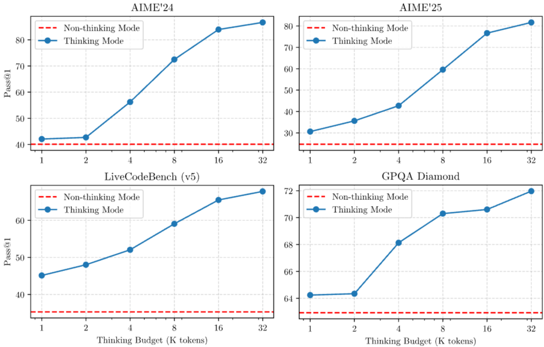
Figure 14.27 Qwen3-235B-A22B performance with thinking budget

Composition of Different Stages

The figure below shows the performance changes of the Qwen3-32B model at different post-training stages:

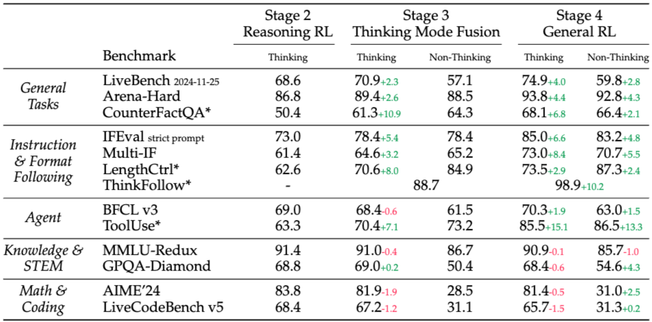
Figure 14.28 Qwen3-32B performance at different stages

It should be noted that general-purpose RLHF slightly decreases math/STEM capabilities.

Qwen 3 proposes Thinking Mode Fusion, attempting to fuse "thinking" and "non-thinking" modes in one model:

• Training: Mix data with <think> and data that directly outputs answers.
• Effect: Users can control whether the model performs long reasoning through the Prompt.
• Test-time Compute: The trade-off between computation amount and performance can be dynamically adjusted during the inference stage by truncating the <think> process.