Chapter 3: PyTorch and Resource Accounting

In Chapter 2 we discussed tokenization. This chapter dives into the mechanics of model training. We won't cover the Transformer architecture directly (that's the next chapter); instead, we'll build simple linear models to master the "primitives" common to training any deep learning model.

Core Objectives:

Mechanics: Master PyTorch fundamentals (bottom-up: tensors → model building → optimizer → training loop).
Mindset: Develop the habit of resource accounting. You need to know how much memory (GB) and compute (FLOPs) each line of code consumes.
Intuitions: Understand why large models require specific hardware and algorithm optimizations.

3.1 Why Do We Need Resource Accounting?

In LLM training, resource consumption directly translates to time and cost. Let's understand through two practical scenarios.

3.1.1 Scenario 1: Time Estimation

Problem: As an AI engineer, your boss asks: "On 1024 H100 GPUs, training a 70B (70 billion parameter) model on 15T (15 trillion) tokens — roughly how long will it take?"

If you rush to write code to test this, you might not get results for days or even months. We need to learn "napkin math" — quick estimation.

Step 1: Calculate total work FLOPs (Floating Point Operations) measure computational complexity — the total count of floating-point additions, multiplications, etc. required during algorithm or model execution. Training a model is essentially performing floating-point operations. An empirical formula:

Total Compute \approx 6 \times Parameters \times Tokens

Why 6×?
Forward Pass: Computing once ≈ $2 \times$ parameters (multiply + add).
Backward Pass: Computing gradients ≈ 2× the forward pass workload, i.e., $4 \times$ parameters.

Plugging in: $6 \times (70 \times 10^{9}) \times (15 \times 10^{12}) \approx 6.3 \times 10^{24} FLOPs$

Step 2: Calculate hardware throughput

Checking the NVIDIA H100 whitepaper, its FP16/BF16 peak throughput is approximately 1979 TFLOPS (trillion floating-point operations per second).

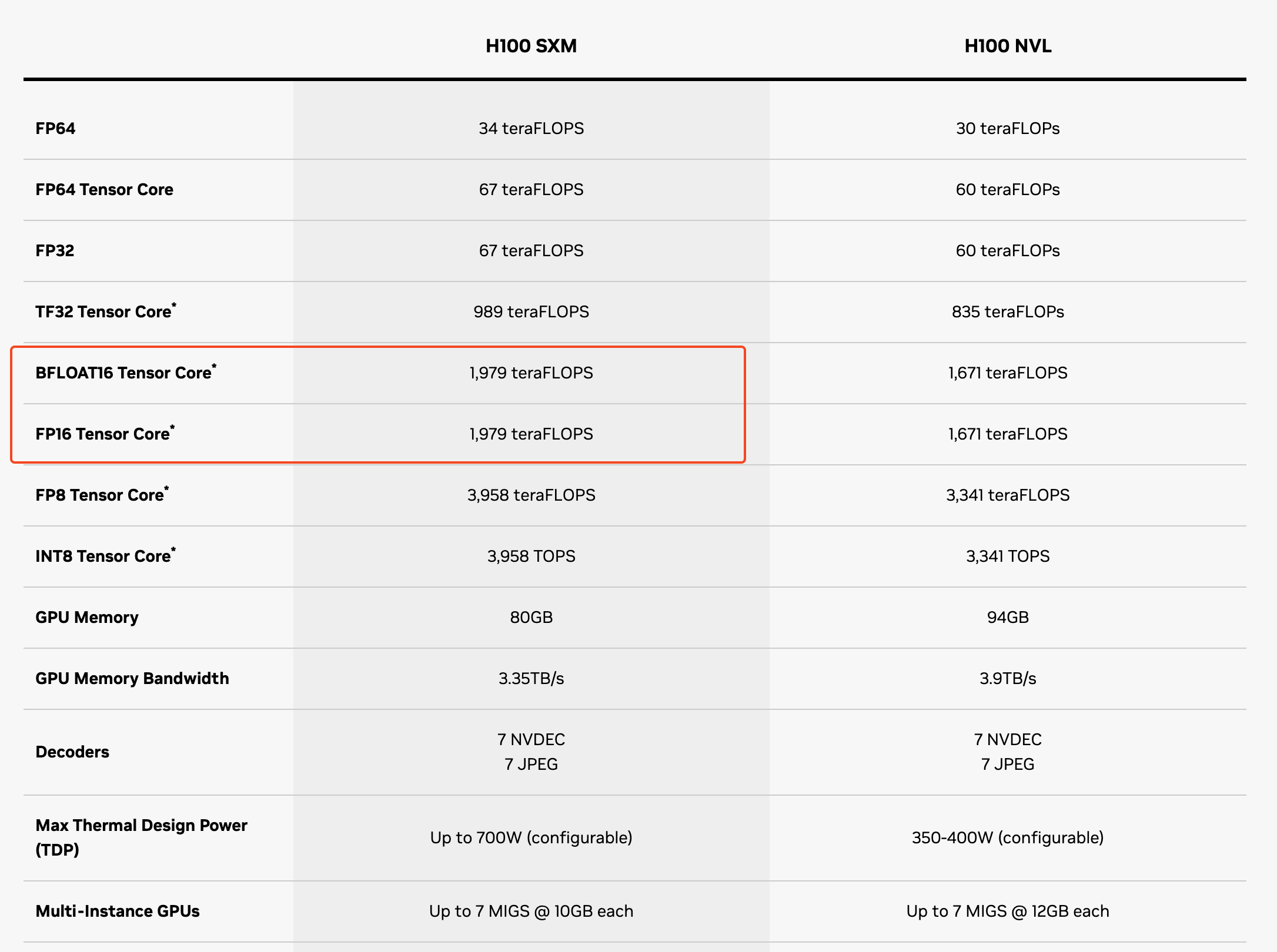
Figure 3.1 H100 Specifications

However, this value is the theoretical maximum computational throughput achievable by an NVIDIA H100 GPU using FP16 or BF16 data types with structured sparsity enabled. For our ordinary dense model training (standard LLaMA-1 through LLaMA-3 series, Qwen3-0.6B/1.7B/4B/8B/14B/32B, etc.), the theoretical peak is approximately halved, around 990 TFLOPS.

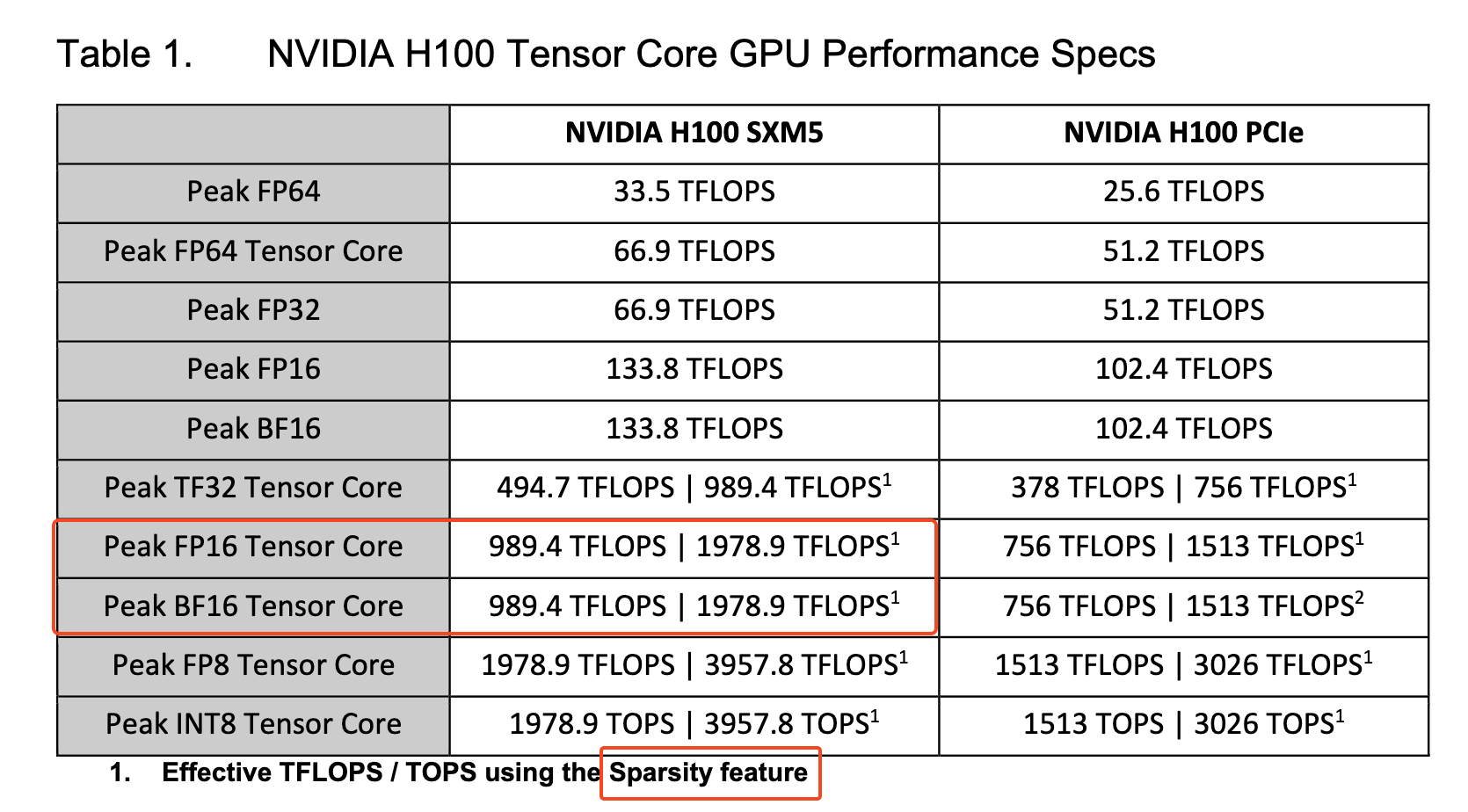
Figure 3.2 H100 Performance Details

Structured sparsity is a model compression method that typically prunes dense models at 50% sparsity (in n:m format, meaning out of m consecutive weights, n must be pruned — types include 2:4, 4:8, 8:16). There's also a more flexible unstructured pruning method that can prune by percentage, but typically performs worse than structured pruning.

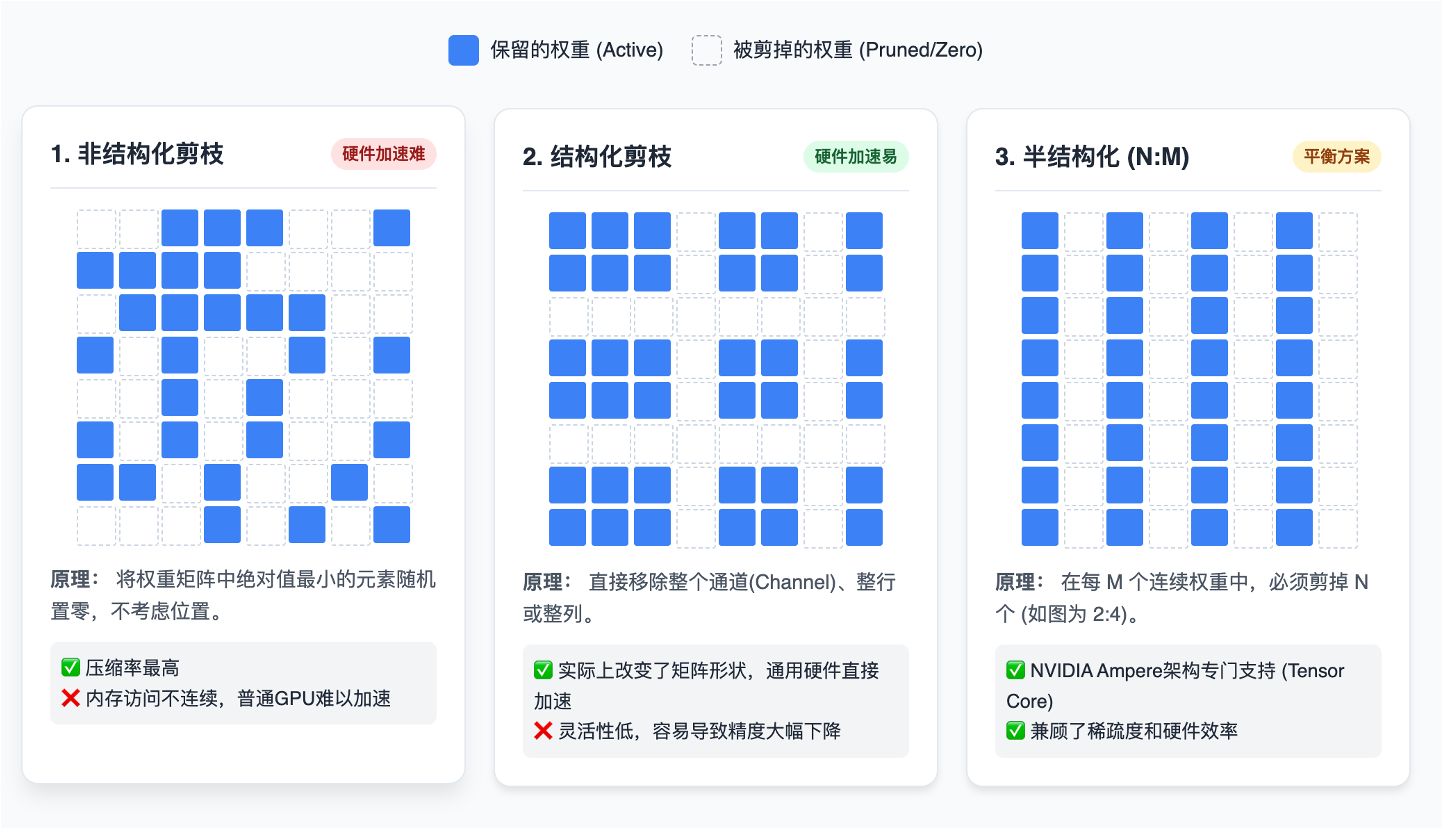
Figure 3.3 Introduction to Pruning Methods

The above 990 TFLOPS is the H100's theoretical peak, but when actually running models, due to various software and hardware overheads, you almost never achieve 100% MFU (Model FLOPs Utilization). Typically, 30%-60% utilization is more realistic for estimation. Let's take 50% for subsequent estimates.

Per-GPU effective: $(990 \times 10^{12}) \times 0.5 \approx 5 \times 10^{14} FLOPS$
1024 GPUs total: $\approx 5 \times 10^{17} FLOPS$

Step 3: Get the result

Time = \frac{Total Work}{Total Throughput} = \frac{6.3 \times 10^{24}}{5 \times 10^{17}} \approx 1.26 \times 10^{7} seconds \approx 146 days

This is a massive engineering project. Without optimization, it would take nearly five months to train — and that's assuming training continues without interruption.

3.1.2 Scenario 2: Memory Estimation

Problem: On 8×H100 GPUs, using the AdamW optimizer (naive implementation — all data in FP32 without mixed precision or compression), what's the largest model you can train?

Many beginners think: 8×80GB = 640GB. FP32 = 4 bytes/parameter. So $640 G B / 4 = 160 B$ parameters? Wrong!

During training, memory stores more than just parameters:

Gradients: Same size as parameters, 4 bytes each
Optimizer States: For example, the commonly used AdamW optimizer needs to store each parameter's first moment estimate (exponential moving average of gradients) and second moment estimate (exponential moving average of squared gradients)

Therefore, each parameter consumes approximately 16 bytes during training:

Parameters (FP32): 4 bytes
Gradients (FP32): 4 bytes
Optimizer States (FP32): 8 bytes (2 variables × 4 bytes)

Max Parameters = \frac{640 \times 10^{9} bytes}{16 bytes/param} \approx 40 billion (40B)

Important caveat: This calculation ignores activation memory (which depends on batch size and sequence length), so it's only a theoretical upper bound. The actual model you can train will be smaller. Activations are the outputs of each layer during forward propagation — as data flows through the network, each matrix multiplication or nonlinear function produces a batch of intermediate results, and these intermediate results are the activations.

3.2 Tensors

Tensors are the fundamental building blocks storing everything in deep learning, including:

Data
Model parameters
Gradients
Optimizer states
Activations

All exist as tensors. For example, in DeepSeek V3.2, all parameters are stored as tensors in the model files:

3.2.1 Tensor Basics

PyTorch provides various methods for creating tensors:

python

x = torch.tensor([[1., 2, 3], [4, 5, 6]])  # From Python list
x = torch.zeros(4, 8)        # 4×8 zero matrix
x = torch.ones(4, 8)         # 4×8 all-ones matrix
x = torch.randn(4, 8)        # 4×8 random normal distribution
x = torch.empty(4, 8)        # Uninitialized 4×8 matrix
nn.init.trunc_normal_(x, mean=0, std=1, a=-2, b=2)  # Truncated normal init, values outside [-2,2] resampled

Tensor Rank: The rank of a tensor is its number of dimensions:

python

x = torch.zeros(4)           # Rank 1 tensor (vector), shape (4,)
x = torch.zeros(4, 8)        # Rank 2 tensor (matrix), shape (4, 8)
x = torch.zeros(4, 8, 2)     # Rank 3 tensor, shape (4, 8, 2)

In Transformers, rank-4 tensors are common:

python

B, S, H, D = 32, 16, 16, 64  # Batch size, Seq length, Heads, Hidden dim per head
x = torch.zeros(B, S, H, D)

3.2.2 Tensor Operations

Most tensors are created by performing operations on other tensors; each operation consumes a certain amount of memory and computational resources.

Tensor Views

Many operations simply provide a different "view" of a tensor. This does not create a copy, so modifications in one tensor affect the other.

python

x = torch.tensor([[1., 2, 3], [4, 5, 6]])
y = x[0]                # Get row 0
y = x[:, 1]             # Get column 1
y = x.view(3, 2)        # Reshape to 3×2
y = x.transpose(1, 0)   # Transpose
assert same_storage(x, y)  # Verify shared storage
x[0][0] = 100; assert y[0][0] == 100  # Value also modified

Note: Not all views are "contiguous." When a view's data isn't stored sequentially in memory, it's non-contiguous.

A transposed tensor is non-contiguous:

python

x = torch.tensor([[1., 2, 3], [4, 5, 6]])
y = x.transpose(1, 0)
assert not y.is_contiguous()  # Non-contiguous tensor

You cannot directly perform certain operations (like view) on non-contiguous tensors. If you need further operations, call .contiguous() first:

python

y = x.transpose(1, 0).contiguous().view(2, 3)
assert not same_storage(x, y)  # Now created new storage

.contiguous() creates a new tensor by copying data sequentially into a new contiguous memory block, ensuring subsequent operations work correctly.

Element-wise Operations

Element-wise operations apply a function independently to each element and return a new tensor of the same shape. This means when you do x.pow(2) or x + x, the operation acts independently on each number in the tensor, without considering row-column relationships.

python

x = torch.tensor([1, 4, 9])
assert torch.equal(x.pow(2), torch.tensor([1, 16, 81]))     # Power
assert torch.equal(x.sqrt(), torch.tensor([1, 2, 3]))        # Square root
assert torch.equal(x.rsqrt(), torch.tensor([1, 1/2, 1/3]))  # Reciprocal sqrt
assert torch.equal(x + x, torch.tensor([2, 8, 18]))          # Element-wise addition
assert torch.equal(x * 2, torch.tensor([2, 8, 18]))          # Scalar multiplication
assert torch.equal(x / 0.5, torch.tensor([2, 8, 18]))        # Scalar division

Finally, we introduce a very useful utility function triu, which is important for computing causal attention masks. In language models, to ensure the model when predicting the j-th word can only see words before position j (i.e., cannot "peek" at future information), this upper triangular matrix is used as a mask. M[i,j] represents the contribution of position i to position j; when i > j (i is after j), the contribution should be 0.

python

x = torch.ones(3, 3).triu()
# Result:
# [[1, 1, 1],
#  [0, 1, 1],
#  [0, 0, 1]]

Matrix Multiplication

Matrix multiplication is the foundation of deep learning. It is the most core and most frequent computational operation in neural networks — whether fully-connected layers, convolutional layers, or attention mechanisms, they all fundamentally rely on matrix operations.

python

x = torch.ones(16, 32)  # 16×32 matrix
w = torch.ones(32, 2)   # 32×2 weight matrix
y = x @ w               # Result: 16×2 matrix
assert y.size() == torch.Size([16, 2])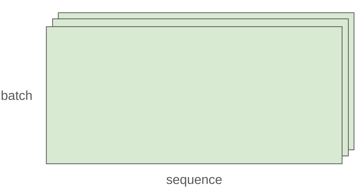

Figure 3.4 Matrix Multiplication

In practice, we rarely process single data samples. For efficiency, we pack multiple samples into a "batch" and compute on the entire batch simultaneously:

python

x = torch.ones(4, 8, 16, 32)  # [batch, seq, features, hidden_dim]
w = torch.ones(32, 2)          # Weight matrix
y = x @ w                      # Matrix multiplication
assert y.size() == torch.Size([4, 8, 16, 2])

PyTorch automatically iterates over the first two dimensions of x (4 and 8), performing matrix multiplication with w on each 16×32 sub-matrix. The final result y has shape (4, 8, 16, 2), where the first two dimensions remain unchanged and the last two change according to matrix multiplication rules.

3.2.3 Optimizing Tensor Operations with Einops

In PyTorch, tensor dimensions are typically [batch, sequence, hidden]. Using native .view() and .transpose() requires keeping track of dimension order — easy to get confused. If you later modify the tensor shape, the code may break.

python

x = torch.ones(2, 2, 3)  # batch, sequence, hidden
y = torch.ones(2, 2, 3)
z = x @ y.transpose(-2, -1)  # Result: (batch, sequence, sequence)

How to solve this? We recommend using jaxtyping to declare dimension semantics first, then einops to manipulate tensors, making code as clear as writing formulas.

1. Naming Dimensions with jaxtyping

python

# Traditional (easy to get dimension order wrong)
x = torch.ones(2, 2, 1, 3)  # batch seq heads hidden

# Jaxtyping style (named dimensions in type annotations)
from jaxtyping import Float
x: Float[torch.Tensor, "batch seq heads hidden"] = torch.ones(2, 2, 1, 3)

jaxtyping's dimension naming (like "batch seq hidden") is primarily "documentation" in the current PyTorch ecosystem — it doesn't automatically enforce at runtime that dimensions actually match the names, but it greatly improves code clarity and reliability. Python's type annotations are optional and non-enforced, primarily used by tools (IDE, mypy) for static analysis rather than runtime checking. Despite not enforcing, jaxtyping brings significant engineering value: when you modify models (e.g., adding a heads dimension), type annotations remind you where updates are needed, and IDEs offer autocompletion, refactoring support, and error highlighting.

2. Using einops.einsum Instead of Matrix Multiply + Transpose

python

from einops import einsum
x: Float[torch.Tensor, "batch seq1 hidden"] = torch.ones(2, 3, 4)
y: Float[torch.Tensor, "batch seq2 hidden"] = torch.ones(2, 3, 4)
# Traditional: z = x @ y.transpose(-2, -1)
z = einsum(x, y, "batch seq1 hidden, batch seq2 hidden -> batch seq1 seq2")
# Dimensions not named in output (hidden) are automatically summed

The ... notation means "any number of leading dimensions," making code applicable to tensors with different shapes.

3. Using einops.reduce Instead of mean(dim=...)

python

from einops import reduce
x: Float[torch.Tensor, "batch seq hidden"] = torch.ones(2, 3, 4)
y = reduce(x, "... hidden -> ...", "mean")  # Instead of x.mean(dim=-1)

4. Using einops.rearrange to Split/Merge Dimensions

python

from einops import rearrange
x: Float[torch.Tensor, "batch seq total_hidden"] = torch.ones(2, 3, 8)
w: Float[torch.Tensor, "hidden1 hidden2"] = torch.ones(4, 4)
# Split total_hidden into heads and hidden1
x = rearrange(x, "... (heads hidden1) -> ... heads hidden1", heads=2)
# Matrix multiply on hidden1
x = einsum(x, w, "... hidden1, hidden1 hidden2 -> ... hidden2")
# Merge dimensions back
x = rearrange(x, "... heads hidden2 -> ... (heads hidden2)")

Despite adding slight syntax overhead, einops' clear dimension naming significantly reduces debugging difficulty, especially in complex model architectures.

3.3 Memory

Tensor memory is determined by two factors:

Element count: The tensor's shape (e.g., a 4×8 matrix has 32 elements)
Data type: Bytes per element

3.3.1 Floating-Point Types

In LLM training, choosing a data type fundamentally involves trading off memory usage, computational speed, and numerical stability. Most tensors we care about (parameters, gradients, activations, optimizer states) are stored as floating-point numbers.

1. Float32 (FP32 / Single Precision)

Figure 3.5 FP32

Specs: 4 bytes (32 bits). Structure: 1 sign + 8 exponent + 23 mantissa bits.
Status: PyTorch default data type, the "gold standard" of scientific computing.
Pros: High numerical precision, wide dynamic range, most stable training, almost no overflow problems.
Cons: Too "luxurious" for large models — 2× the memory of 16-bit formats, and computational throughput on modern GPUs (H100) is far lower than low-precision formats.
Training use: Typically used for storing master weights and optimizer states to ensure no precision loss during gradient accumulation and parameter updates.

2. Float16 (FP16 / Half Precision)

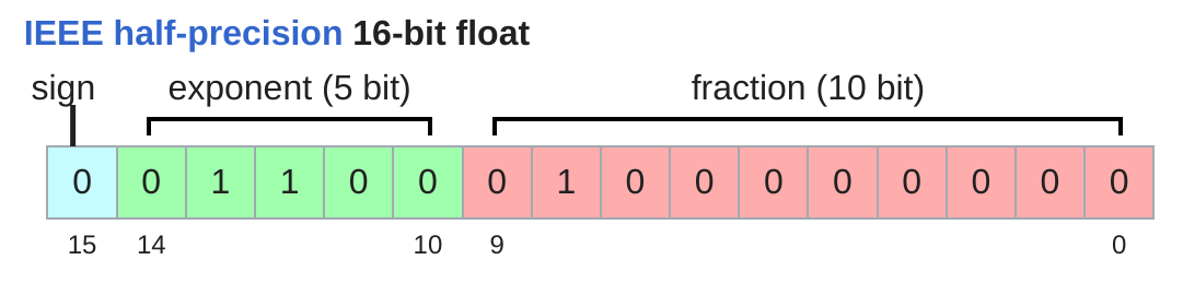
Figure 3.6 FP16

Specs: 2 bytes (16 bits). Structure: 1 sign + 5 exponent + 10 mantissa bits.
Pros: Memory halved vs. FP32, faster computation.
Fatal flaw: Dynamic range too narrow. With only 5 exponent bits, it cannot represent very small numbers (underflow to 0) or very large numbers (overflow to Infinity). For example, values like 1e-8 are treated as 0 in FP16, causing gradient vanishing.
Use: Mainstream for previous-generation GPU (V100) mixed-precision training. Requires complex loss scaling. Being replaced by BF16 in LLM training.

3. BFloat16 (BF16 / Brain Floating Point)

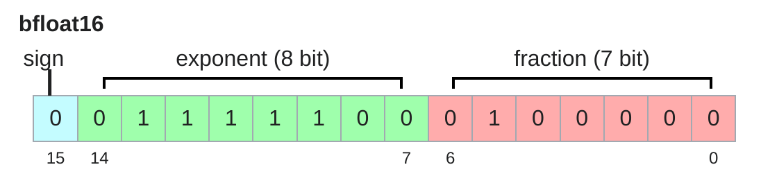
Figure 3.7 BF16

Specs: 2 bytes (16 bits). Structure: 1 sign + 8 exponent + 7 mantissa bits.
Origin: Designed by Google Brain specifically for deep learning.
Design logic: "Prioritize range over precision." Deep learning models are insensitive to the last few decimal places of precision but highly sensitive to value range. BF16 directly truncates FP32's mantissa while retaining the same 8-bit exponent as FP32.
Pros: Same dynamic range as FP32 (no loss scaling needed); memory same as FP16; extremely fast on A100/H100 hardware.
Use: Current absolute mainstream for LLM training. Typically used for activations and the matrix multiplications in forward/backward propagation.

Percy explains: "BF16 sacrifices precision for range. For deep learning, range is far more important than precision because the main threat to numerical stability is overflow/underflow, not insufficient mantissa precision."

4. FP8 (8-bit Floating Point)

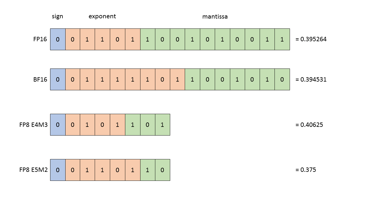
Figure 3.8 FP8

Specs: 1 byte (8 bits).
Variants: E4M3 (4-bit exponent, 3-bit mantissa — slightly higher precision, smaller range); E5M2 (5-bit exponent, 2-bit mantissa — larger range, lower precision).
Pros: Ultimate memory compression and computational throughput.
Hardware limitation: Only natively supported on H100 and newer architectures (with Transformer Engine).
Training use: Currently mainly for inference quantization. Training in FP8 is cutting-edge research — extremely unstable due to low precision.

5. FP4 / NVFP4 (4-bit Floating Point)

In 2025, NVIDIA developed NVFP4, each value only 4 bits! The 16 representable values: -6, -4, -3, -2, -1.5, -1.0, -0.5, 0, 0.5, 1.0, 1.5, 2, 3, 4, 6.

Percy emphasized a key detail: NVFP4 is not simply each value having only 4-bit dynamic range. "If you naively only used these 16 values, you couldn't train effectively. In reality, each value has 4 bits of freedom, but data is divided into blocks, each with a shared scale factor that can amplify or shrink values. This way, individual values actually have more than 4 bits of dynamic range, though the ratio between adjacent values is still constrained by 4 bits."

Using an analogy: within each block you can freely vary within 4-bit precision, while the block's scale factor lets the whole block's values shift to different magnitudes. The cost is you can't have one value very large while its neighbor is very small — they belong to the same block sharing the same scale factor.

Percy distinguishes training vs. inference: for inference, you can quantize a BF16-trained model's weights to 1 or 2 bits; for training, "I don't think anyone has done credible 1-bit training." Nemotron 3 Super (2026) was trained in NVFP4 precision.

Percy also mentions that these low-precision operations are actually done automatically in NVIDIA's software stack, "not something where you create a tensor and call tensor.fp4() — much work happens 'under the hood' beyond direct user control."

🪜 Why BF16 is better than FP16?

In deep learning, we typically don't care about the 10th decimal place of precision, but care deeply about being able to represent very large or very small numbers (dynamic range). FP16's exponent bits are too few, causing frequent NaN or 0 (underflow) during training. BF16 truncates FP32's mantissa while retaining exponent bits, giving it the same value range as FP32, greatly improving training stability.

Different precisions have completely different computation speeds. Percy emphasizes: "GPUs now barely optimize FP32 anymore" — if you do FP32 training now, you'll find it really, really slow because hardware optimization has shifted to BF16 and even FP8.

3.3.2 Tensor Storage Mechanism

In PyTorch, how are tensors actually stored at the low level? PyTorch tensors adopt row-major storage. A tensor itself doesn't directly "contain" data but points to a contiguous memory region with a set of rules (metadata) telling the program how to find the corresponding data based on your requested indices.

python

x = torch.tensor([[0.,1,2,3],[4,5,6,7],[8,9,10,11],[12,13,14,15]])

The answer is strides! Stride is a tuple defining how many elements to "skip" in the underlying storage when moving one unit in each dimension.

python

assert x.stride(0) == 4  # Row dim: moving to next row skips 4 elements
assert x.stride(1) == 1  # Col dim: moving to next col skips 1 element
r, c = 1, 2
index = r * x.stride(0) + c * x.stride(1)  # Position 6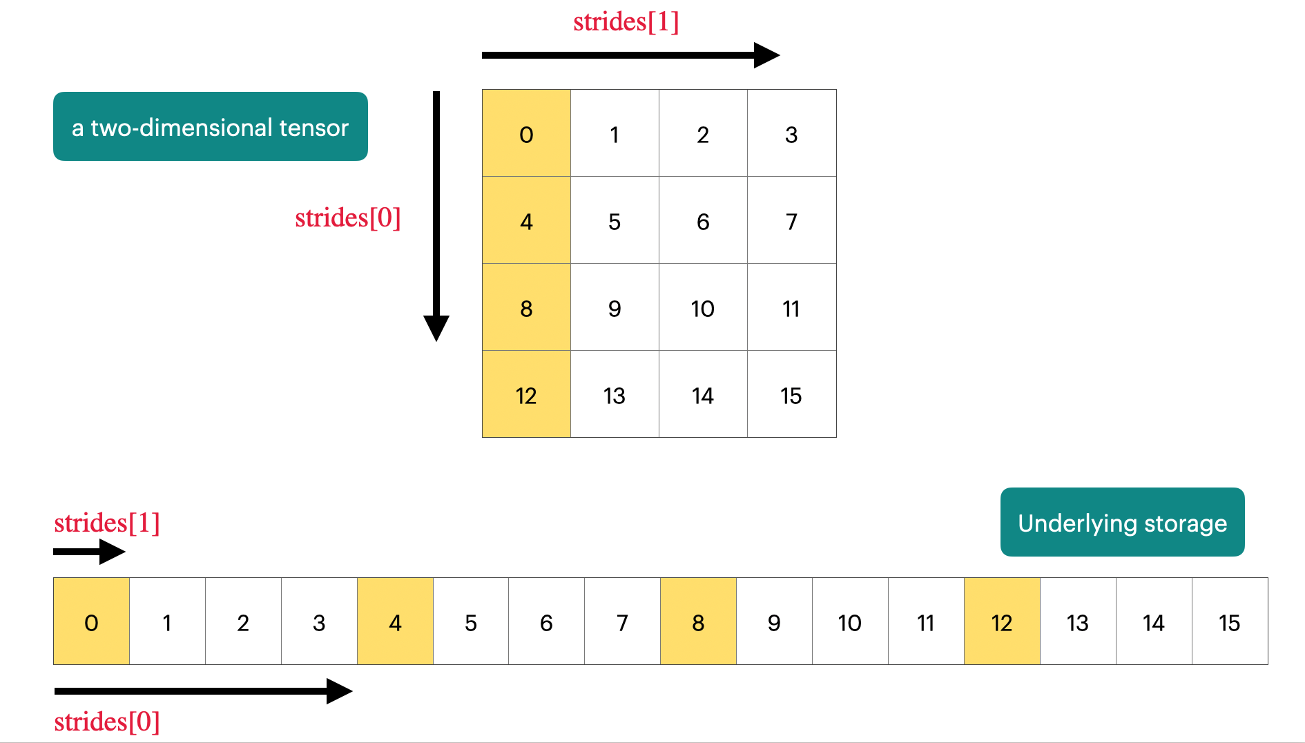

Figure 3.9 Tensor Memory

In one sentence: PyTorch cleverly maps multi-dimensional tensor logical structure to one-dimensional physical memory through the "stride" metadata.

Key point: Many operations (like view, transpose, slice) do not copy data — they only modify the stride. This is called zero-copy and is very efficient. Pitfall: Calling .view() on a transposed tensor may error because the memory is no longer contiguous. You must first call .contiguous(), which triggers data copying (consuming memory and time).

3.3.3 Moving Tensors from CPU to GPU Memory

By default, tensors are stored on CPU memory. To leverage GPU's massive parallelism, we need to move them to GPU.

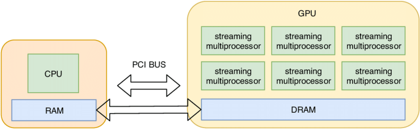
Figure 3.10 CPU-GPU Communication

The left side contains the CPU and system RAM; the right side contains the GPU and its dedicated high-speed DRAM. The GPU internally consists of multiple "streaming multiprocessors" — the source of its parallel computing power. CPU and GPU communicate via PCI bus, typically a performance bottleneck because its bandwidth is far smaller than GPU internal memory bandwidth. Therefore, in practice, we should minimize CPU-GPU data transfers.

python

if not torch.cuda.is_available(): return
num_gpus = torch.cuda.device_count()
for i in range(num_gpus):
    properties = torch.cuda.get_device_properties(i)  # GPU properties
memory_allocated = torch.cuda.memory_allocated()       # Current allocated GPU memory
# Method 1: Move existing tensor
y = x.to("cuda:0")
# Method 2: Create directly on GPU (more efficient, avoids CPU→GPU transfer)
z = torch.zeros(32, 32, device="cuda:0")
# Verify memory allocation
new_memory_allocated = torch.cuda.memory_allocated()
memory_used = new_memory_allocated - memory_allocated
assert memory_used == 2 * (32 * 32 * 4)  # Two 32×32 FP32 matrices

3.4 Compute Efficiency

3.4.1 FLOPs (Floating Point Operations)

A FLOP is a basic arithmetic operation like addition or multiplication. Understanding FLOPs is crucial for performance analysis.

MFU (Model FLOPs Utilization): Actual throughput / Theoretical peak. Real-world MFU is typically 30-60%.

3.4.2 Arithmetic Intensity

Arithmetic intensity = FLOPs / bytes of memory access. This determines whether an operation is compute-bound (limited by GPU compute) or memory-bound (limited by memory bandwidth). For LLMs: attention is memory-bound for short sequences and compute-bound for long sequences; FFN/MLP is typically compute-bound; LayerNorm/RMSNorm is heavily memory-bound.

3.5 Model Building and Training Fundamentals

3.5.1 Parameter Initialization

Now let's write code. We'll build a simple Deep Linear Network and manually implement the optimizer.

Storing Model Parameters

In PyTorch, trainable model parameters are encapsulated as nn.Parameter objects:

python

w = nn.Parameter(torch.randn(input_dim, output_dim))

nn.Parameter is a subclass of torch.Tensor, so it "behaves like a tensor" and supports all tensor operations. It has a .data attribute for accessing its underlying torch.Tensor data.

The Importance of Initialization and Common Methods

If you directly use torch.randn for standard Gaussian initialization, as the number of layers deepens, values become very large (explosion) or very small (vanishing).

python

x = nn.Parameter(torch.randn(input_dim)) # Input vector
output = x @ w # Output vector

When input_dim = 16384, the output magnitude is approximately 18.9 — a very large value. Such large values amplify layer by layer, causing gradient explosion, making training extremely unstable or even impossible to converge.

To overcome this, we need an initialization method insensitive to the input dimension. The solution is Xavier initialization (paper, StackExchange community). By dividing by $\sqrt{input dimension}$ to scale weights, we maintain numerical stability.

python

w = nn.Parameter(torch.randn(input_dim, output_dim) / np.sqrt(input_dim))

After scaling, each element of the output becomes stable within a small range, no longer growing with input_dim.

Even with Xavier initialization, since the tails of the normal distribution are unbounded, extreme values (outliers) can still occur. The solution is to use a truncated normal distribution, constraining generated random numbers within a reasonable range (e.g., [-3, 3]).

python

w = nn.Parameter(nn.init.trunc_normal_(torch.empty(input_dim, output_dim), 
                                      std=1 / np.sqrt(input_dim), 
                                      a=-3, b=3))

3.5.2 Building Custom Models with PyTorch

This section covers how to build a custom deep linear model from scratch in PyTorch. It demonstrates using nn.Parameter to define learnable parameters and composing them to create a simple neural network.

Defining the model structure. Here we define a custom model class called Cruncher — a "deep linear model" with num_layers hidden layers and one output layer.

python

D = 64 # Dimension
num_layers = 2
model = Cruncher(dim=D, num_layers=num_layers)

The Cruncher class combines multiple Linear layers to form a deeper network. In __init__, nn.ModuleList creates a list of num_layers Linear layers. Each Linear layer has input and output dimensions both equal to dim, meaning they are "identity" transformations, but the internal weights are learnable.

python

class Cruncher(nn.Module):
    def __init__(self, dim: int, num_layers: int):
        super().__init__()
        self.layers = nn.ModuleList([
            Linear(dim, dim)
            for i in range(num_layers)
        ])
        self.final = Linear(dim, 1)  # Create a final Linear layer mapping dim-dimensional features to 1-dimensional scalar output
    def forward(self, x: torch.Tensor) -> torch.Tensor:
        # Apply linear layers
        B, D = x.size()
        for layer in self.layers:
            x = layer(x)
        # Apply final head
        x = self.final(x)
        assert x.size() == torch.Size([B, 1])
        # Remove the last dimension
        x = x.squeeze(-1) # Remove the last dimension (the size-1 dimension), making the final output a 1D tensor (B,), more intuitive for "predicted values" (e.g., one score per sample)
        assert x.size() == torch.Size([B])
        return x

The Linear class implements the most fundamental building block in neural networks — the linear layer (also called fully-connected or dense layer).

python

class Linear(nn.Module):
    """Simple linear layer."""
    def __init__(self, input_dim: int, output_dim: int):
        super().__init__()
        self.weight = nn.Parameter(torch.randn(input_dim, output_dim) / np.sqrt(input_dim))
    def forward(self, x: torch.Tensor) -> torch.Tensor:
        return x @ self.weight

Inspecting model parameters. Using model.state_dict() returns a dictionary containing the names and values of all learnable parameters (nn.Parameter) in the model.

python

param_sizes = [
    (name, param.numel())  # param.numel(): returns the total number of elements in this parameter tensor
    for name, param in model.state_dict().items()
]
assert param_sizes == [
    ("layers.0.weight", D * D),
    ("layers.1.weight", D * D),
    ("final.weight", D),
]

Moving the model to GPU. In actual training, to leverage GPU parallel computation, both the model and data need to be moved to the GPU. The get_device() function automatically selects an available GPU or CPU.

python

device = get_device()
model = model.to(device)

Running the model on data. Create a batch of B=8 random input data x, call model(x) for forward propagation, and obtain output y. Verify that output y has shape (B,) — each sample corresponds to one scalar output.

python

B = 8 # Batch size
x = torch.randn(B, D, device=device)
y = model(x)
assert y.size() == torch.Size([B])

3.5.3 Managing Randomness for Reproducibility

Sources of Randomness

Randomness appears in many places in deep learning:

Parameter initialization: model weights are typically sampled from random distributions (e.g., normal distribution).
Dropout: randomly "turns off" a subset of neurons during training.
Data ordering: data loaders typically shuffle data order.
Others: data augmentation, momentum in optimizers, etc.

These sources of randomness cause different results each time you run the code — a huge obstacle when debugging and comparing different models. To ensure experiment reliability and comparability, we need to make program behavior deterministic.

Setting Random Seeds

Three main libraries need separate random seed setting, typically done once at the start of the program.

1. PyTorch

Set the seed for PyTorch's own random number generator, affecting all operations using torch.randn, torch.randint, etc.

python

seed = 0
torch.manual_seed(seed)

2. NumPy

Many data preprocessing operations (e.g., data loading, splitting) depend on NumPy's random functions, so its seed also needs separate setting.

python

import numpy as np
np.random.seed(seed)

3. Python Standard Library (random)

Python's built-in random module is also commonly used for data shuffling and needs seed setting.

python

import random
random.seed(seed)

Key tip: While you could set different seeds for each random source (e.g., fix initialization but allow data variation), in most cases, the simplest and safest approach for full reproducibility is to set all three seeds to the same value.

3.5.4 Data Loading

In language modeling, input data is typically integer sequences processed by a tokenizer. For example, the sentence "Hello world" might be encoded as [1, 2]. For convenient processing, these integer sequences are usually saved as NumPy array files (.npy format).

python

orig_data = np.array([1, 2, 3, 4, 5, 6, 7, 8, 9, 10], dtype=np.int32)
orig_data.tofile("data.npy") # Save array to file

For extremely large datasets like LLaMA's 2.8TB training data, it's impossible to load everything into memory. The solution is to use numpy.memmap to create a "memory-mapped" object.

python

data = np.memmap("data.npy", dtype=np.int32) # Create memory map
assert np.array_equal(data, orig_data) # Verify loaded data is correct

The data object itself doesn't contain data — it's a "pointer" to the file on disk. When you access data[0] or data[1:10], the system loads only that portion from disk into memory on demand. This approach dramatically saves memory, allowing you to process datasets far larger than available RAM.

In actual training, we don't operate on the entire dataset directly but use a "data loader" to generate training batches.

python

B = 2  # Batch size — how many samples to process in one training step
L = 4  # Sequence length — how many tokens each sample contains
x = get_batch(data, batch_size=B, sequence_length=L, device=get_device())
assert x.size() == torch.Size([B, L]) # Verify output tensor shape

Calling get_batch randomly samples B starting positions from data, then extracts a sequence of length L after each position, ultimately returning a tensor x of shape (B, L).

Let's examine the internal logic of the get_batch function:

python

def get_batch(data: np.array, batch_size: int, sequence_length: int, device: str) -> torch.Tensor:
    # Randomly sample starting positions
    start_indices = torch.randint(len(data) - sequence_length, (batch_size,)) # Use torch.randint to randomly generate batch_size starting indices in [0, len(data) - sequence_length]. This ensures each sequence can be fully extracted without going out of bounds
    assert start_indices.size() == torch.Size([batch_size]) # Verify correct index count

    # Extract data based on starting indices
    x = torch.tensor([data[start:start + sequence_length] for start in start_indices]) # Iterate over each starting position in start_indices, slicing a subsequence of length sequence_length from data. Finally convert these subsequences into a PyTorch tensor x with shape (batch_size, sequence_length)
    assert x.size() == torch.Size([batch_size, sequence_length])

    # Pinned Memory optimization
    if torch.cuda.is_available():
        x = x.pin_memory()

    # Asynchronous data transfer
    x = x.to(device, non_blocking=True)

This function's core purpose is to randomly extract batch_size sequences from a large one-dimensional array data, each of length sequence_length.

Parameter descriptions:

data: input data, a NumPy array, typically integer sequences processed by a tokenizer.
batch_size: number of sequences to sample.
sequence_length: length of each sequence.
device: target device (e.g., "cuda:0" or "cpu").

Pinned Memory optimization: By default, CPU tensors are stored in "paged memory." When transferring data from CPU to GPU, the OS must first copy the data to a "non-pageable" memory region, then send it to the GPU via PCIe bus. This process is synchronous and blocks the current process. By calling .pin_memory(), we explicitly mark the CPU tensor as "pinned" — its physical memory address is fixed and won't be swapped out to disk by the OS. This allows the GPU driver to directly access this memory without extra copy steps.

Asynchronous transfer: Setting non_blocking=True tells PyTorch that data transfer can happen asynchronously in the background without blocking the current Python thread.

By combining "pinned memory" and "asynchronous transfer," we achieve an efficient pipelining:

Process the current batch on GPU.
Simultaneously load the next batch on CPU (e.g., reading from disk or memory-mapped file).

This parallelization significantly reduces GPU idle time, dramatically improving overall training throughput.

For more on data loading optimization, see How to Optimize Data Transfers in CUDA C/C++ and Tricks to Speed Up Data Loading with PyTorch.

3.5.5 Optimizer

Common Optimizers Overview

SGD (Stochastic Gradient Descent): The most basic optimizer — directly multiplies gradient by learning rate to update parameters.
Momentum: Adds a "momentum" term on top of SGD — the exponential moving average of gradients — helping accelerate convergence and reduce oscillation.
AdaGrad: Adjusts each parameter's learning rate based on the historical sum of squared gradients — friendlier to sparse features.
RMSProp: An improvement over AdaGrad, using exponentially weighted average of squared gradients instead of simple accumulation, preventing learning rate from decaying too early.
Adam: Combines ideas from RMSProp and Momentum — currently the most popular optimizer.

Let's take AdaGrad as an example (although AdamW is more commonly used today, the principle is similar). The optimizer must not only update parameters but also remember each parameter's historical gradient information (state).

python

class AdaGrad(torch.optim.Optimizer):
    def step(self):
        for group in self.param_groups:
            for p in group['params']:
                grad = p.grad.data
                # Get state (sum of squared gradients)
                state = self.state[p]
                if 'sum_squared_grad' not in state:
                    state['sum_squared_grad'] = torch.zeros_like(p.data)
                
                # Update state: accumulate squared gradients
                state['sum_squared_grad'] += grad ** 2
                
                # Update parameter: divide by sqrt(state)
                std = state['sum_squared_grad'].sqrt() + 1e-10
                p.data -= group['lr'] * grad / std

Using the Optimizer

Instantiating and using an AdaGrad optimizer in PyTorch:

python

# Instantiate optimizer
optimizer = AdaGrad(model.parameters(), lr=0.01) # model.parameters(): passes all learnable parameters in the model to the optimizer

# Compute gradients
loss.backward() # Compute gradients of the loss function with respect to all parameters

# Execute one update step
optimizer.step() # Update model parameters based on gradients and optimizer internal state

Freeing memory (optional)

Before each iteration, previously computed gradients must be cleared, otherwise they accumulate. When calling zero_grad, setting set_to_none=True is a more efficient memory management approach — it sets gradient pointers to None rather than zeroing them, saving memory.

python

optimizer.zero_grad(set_to_none=True)

Optimizer Under the Hood

This section demonstrates custom implementations of SGD and AdaGrad optimizers, giving you deep insight into their internal workings.

The most basic gradient descent algorithm:

python

class SGD(torch.optim.Optimizer):
    def __init__(self, params: Iterable[nn.Parameter], lr: float = 0.01):
        super(SGD, self).__init__(params, dict(lr=lr)) # Call parent Optimizer's init, storing learning rate lr in the parameter group dictionary

    def step(self):
        for group in self.param_groups: # Iterate over all parameter groups (typically one group)
            lr = group["lr"]
            for p in group["params"]: # Iterate over each parameter p in this group
                grad = p.grad.data  # Get this parameter's gradient grad
                p.data -= lr * grad # Update parameter

AdaGrad's core idea is "adaptive learning rate" — dynamically adjusting each parameter's learning rate based on its historical gradient information, performing better on sparse data.

python

class AdaGrad(torch.optim.Optimizer):
    def __init__(self, params: Iterable[nn.Parameter], lr: float = 0.01):
        super(AdaGrad, self).__init__(params, dict(lr=lr))

    def step(self):
        for group in self.param_groups:
            lr = group["lr"]
            for p in group["params"]:
                state = self.state[p] # Get optimizer state
                grad = p.grad.data

                g2 = state.get("g2", torch.zeros_like(grad)) # Get or initialize sum of squared gradients
                g2 += torch.square(grad) # Accumulate current gradient squared
                state["g2"] = g2 # Update state

                p.data -= lr * grad / torch.sqrt(g2 + 1e-5) # Update parameter

state: a dictionary storing each parameter's optimizer state. For AdaGrad, the state is g2 — the cumulative sum of historical squared gradients.
state.get("g2", torch.zeros_like(grad)): if g2 doesn't exist, initialize as all-zero tensor; if it exists, retrieve its value.
g2 += torch.square(grad): accumulate the square of the current gradient into g2.
p.data -= lr * grad / torch.sqrt(g2 + 1e-5): update the parameter. The division makes the learning rate decrease as g2 grows, penalizing frequently updated parameters while giving larger step sizes to sparsely updated ones. 1e-5 prevents division by zero.

3.5.6 Resource Accounting

This section teaches how to estimate the memory and compute resources needed during model training.

Memory Footprint Analysis

For a deep linear model, total memory requirements consist of four components:

Parameters: the number of all learnable weights in the model.
Activations: intermediate results produced during forward propagation, which must be saved for backpropagation.
Gradients: gradients computed during backpropagation, equal in count to parameters.
Optimizer States: additional state information maintained by the optimizer (e.g., AdaGrad's g2), also equal in count to parameters.

Assuming all data uses float32 format (4 bytes per element), total memory is:

total_memory = 4 * (num_parameters + num_activations + num_gradients + num_optimizer_states)

Parameter count: (D * D * num_layers) + D
Activation count: B * D * num_layers (activations saved per batch, per sample, per layer)
Gradient count: num_parameters
Optimizer state count: num_parameters

Important note: This is a simplified model. In actual Transformer models, memory usage is more complex due to attention mechanisms and other structures, but the basic framework remains the same.

Compute (FLOPs) Analysis

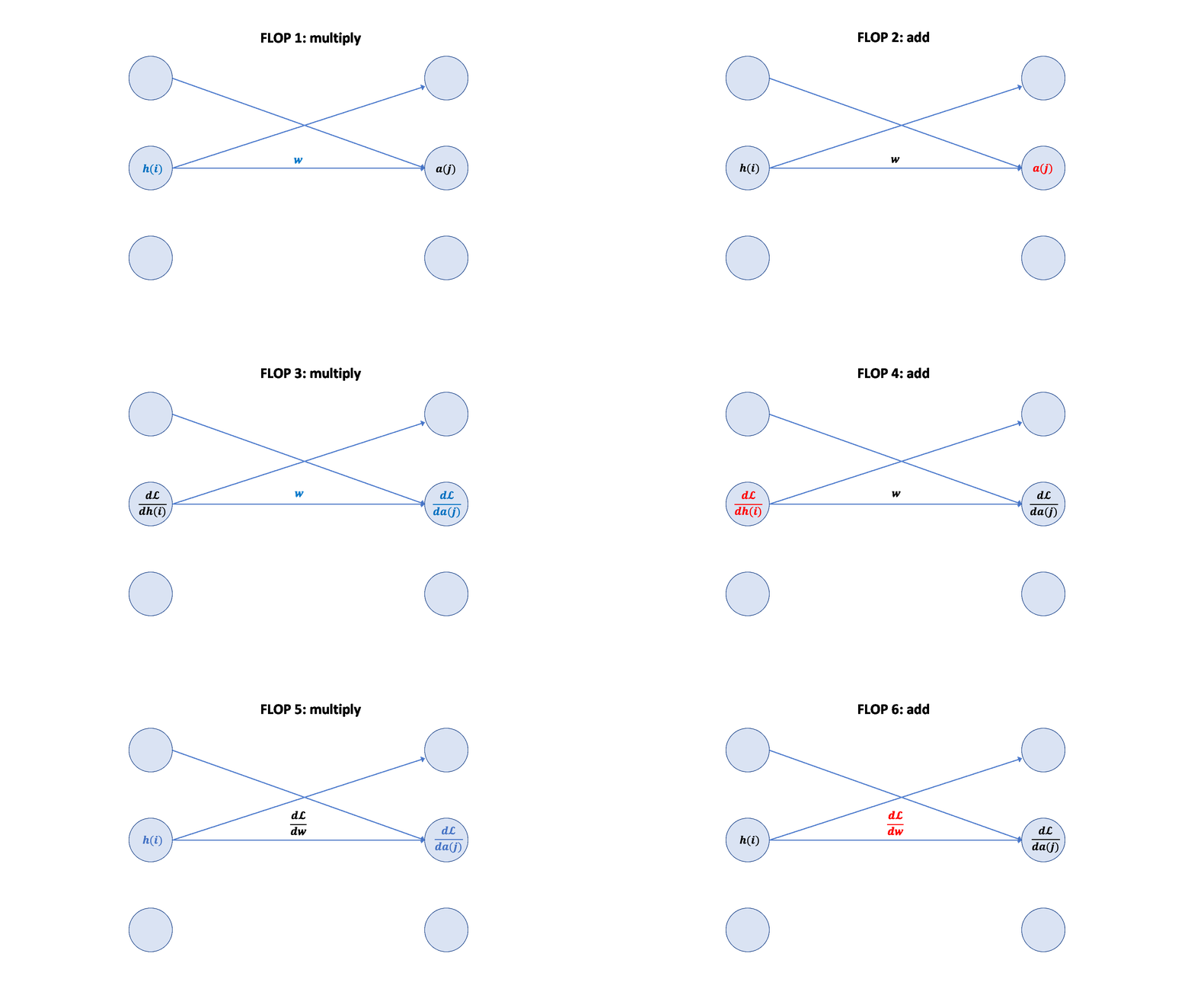
Figure 3.11 Backward Gradient Propagation

From earlier sections, we know that training once (forward + backward) has total FLOPs ≈ 6 × (data count) × (parameter count). Therefore, for one training step:

flops = 6 * B * num_parameters

Transformer processing is more complex, but the principle is the same. In Assignment 1, you'll be asked to complete its memory and compute analysis. These two blog posts will help:

3.5.7 Training Loop: Integrating All Components

This section presents a complete, from-scratch deep learning training loop. Using a simple linear regression task as an example, it clearly demonstrates how to integrate all previously learned components — data generation, model construction, optimizer, forward propagation, backpropagation, and parameter updates — into a runnable training pipeline.

python

def train_loop():
    # Data generation
    D = 16
    true_w = torch.arange(D, dtype=torch.float32, device=get_device()) # Create a true weight vector [0, 1, 2, ..., 15]

    # Data loader for generating training batches
    def get_batch(B: int) -> tuple[torch.Tensor, torch.Tensor]:
        x = torch.randn(B, D).to(get_device()) # Randomly sample B D-dimensional input samples from standard normal distribution
        true_y = x @ true_w # Compute the corresponding "true labels" based on true_w, i.e., y = x @ w_true
        return (x, true_y) # Serve as model input and target output

    # Execute training
    train("simple", get_batch, D=D, num_layers=0, B=4, num_train_steps=10, lr=0.01)
    # Hyperparameter tuning
    train("simple", get_batch, D=D, num_layers=0, B=4, num_train_steps=10, lr=0.1) # Observe the effect of different learning rates by changing lr from 0.01 to 0.1

The train() function implements the standard deep learning training steps in detail:

python

def train(name: str, get_batch,
          D: int, num_layers: int,
          B: int, num_train_steps: int, lr: float):

    # Initialize model and optimizer
    model = Cruncher(dim=D, num_layers=0).to(get_device())
    optimizer = SGD(model.parameters(), lr=lr)

    # Main training loop
    for t in range(num_train_steps): # Loop num_train_steps times; each iteration is called a "training step"
        # Get data
        x, y = get_batch(B=B) # Get input x and target output y for the current batch

        # Forward propagation (compute loss)
        pred_y = model(x)
        loss = F.mse_loss(pred_y, y) # Compute Mean Squared Error between predicted pred_y and true y, as the loss value

        # Backpropagation (compute gradients)
        loss.backward() # Call loss.backward() to trigger automatic differentiation, computing gradients of the loss with respect to all model parameters, storing them in .grad attributes
        
        # Update parameters
        optimizer.step() # Update model parameters based on computed gradients and optimizer update rules (SGD here)
        optimizer.zero_grad(set_to_none=True) # Clear previous step's gradients, preparing for the next iteration

train() function parameter descriptions:

"simple": experiment name.
get_batch: data generation function.
D=16: input dimension.
num_layers=0: model layers = 0, meaning this is a single-layer linear model.
B=4: batch size.
num_train_steps=10: number of training steps.
lr=0.01: learning rate.

3.5.8 Checkpointing

Large language model training takes extremely long — crashes or interruptions are almost inevitable during the process. We need a mechanism to save progress so we can resume from the interruption point rather than starting from scratch.

Why Do We Need Checkpoints?

Long training times: Training a large language model can take days, weeks, or even months.
System instability: Hardware failures, software errors, power outages, human operational mistakes, etc., can all cause unexpected training termination.
Avoiding loss: Without any backup, a single crash means all prior computation and time are wasted.

Therefore, periodically saving "checkpoints" is a fundamental safeguard for ensuring project progress.

What Does a Checkpoint Contain?

To fully restore training, a checkpoint must include all necessary state information. It primarily consists of two core parts:

Model parameters: This is the model's core, containing the current values of all learnable weights (nn.Parameter). model.state_dict() returns a dictionary where keys are parameter names and values are the corresponding tensor data.
Optimizer state (optimizer.state_dict()): This is a part many people overlook but is extremely critical. The optimizer (e.g., Adam, AdaGrad) stores not only the current learning rate but also maintains some internal state variables. For example:
- Adam: stores moving averages of momentum and variance.
- AdaGrad: stores the cumulative sum of historical squared gradients.

If only model parameters are saved without optimizer state, the optimizer will start from zero when training resumes, causing discontinuous training, performance degradation, and potentially failure to converge.

How to Save and Load Checkpoints?

Saving a Checkpoint

python

# 1. Create a dictionary containing model and optimizer states
checkpoint = {
    "model": model.state_dict(),
    "optimizer": optimizer.state_dict(),
}

# 2. Use torch.save to serialize the dictionary and save to disk file
torch.save(checkpoint, "model_checkpoint.pt") # Filenames typically use .pt or .pth extension

Loading a Checkpoint

python

# 1. Load the saved dictionary from disk file
loaded_checkpoint = torch.load("model_checkpoint.pt")

# 2. (Subsequent steps) Load state back into model and optimizer
# model.load_state_dict(loaded_checkpoint["model"])
# optimizer.load_state_dict(loaded_checkpoint["optimizer"])

Note: The above code only shows the loading step. A complete restoration flow also requires calling load_state_dict() methods to apply the loaded data onto the corresponding objects.

3.5.9 Mixed Precision Training

Mixed Precision Training Overview

Problem: FP32 enables stable training but uses too much memory; FP16/BF16 saves memory but has numerical instability risks. How to balance "high-precision stability" and "low-precision efficiency"?

Solution: Mixed Precision Training (Mixed Precision Training, 2017)

The solution is to adopt a mixed precision strategy. Use float32 by default for ensuring precision in critical computations. Where possible, use {bfloat16, fp8} to leverage their efficient memory and compute characteristics. A classic mixed precision training scheme:

Forward Pass: Use bfloat16 or fp8. This includes all intermediate activations. Since activations typically don't require extremely high precision, using low precision significantly saves memory.
Everything else: Use float32. This includes model parameters, gradients, and optimizer states. These are the core of training and need higher precision to ensure numerical stability and convergence.

Core idea: Use low precision for "high-consumption but precision-tolerant" parts (activations), and high precision for "precision-sensitive" parts (parameters and gradients).

Tools for Automatic Mixed Precision Training

Here we introduce two main tool libraries that can automatically implement mixed precision training:

PyTorch AMP library (Automatic Mixed Precision): PyTorch provides an Automatic Mixed Precision (AMP) library that automatically converts safe operations (like matrix multiplication) to bf16 while keeping dangerous operations (like exp, softmax) in fp32:

python

with torch.amp.autocast("cuda", dtype=torch.bfloat16):
    x = torch.zeros(4, 8)  # Automatically created in bf16

Reference: PyTorch AMP Documentation

NVIDIA Transformer Engine: This is a library specifically optimized for Transformer models, supporting FP8 precision in core operations like matrix multiplication. The goal is to achieve end-to-end FP8 training — using FP8 throughout the entire training process to achieve extreme performance and efficiency. — FP8-LM: Training FP8 Large Language Models

3.6 Arithmetic Intensity and Roofline Analysis

3.6.1 Compute Isn't Just About "Computing"

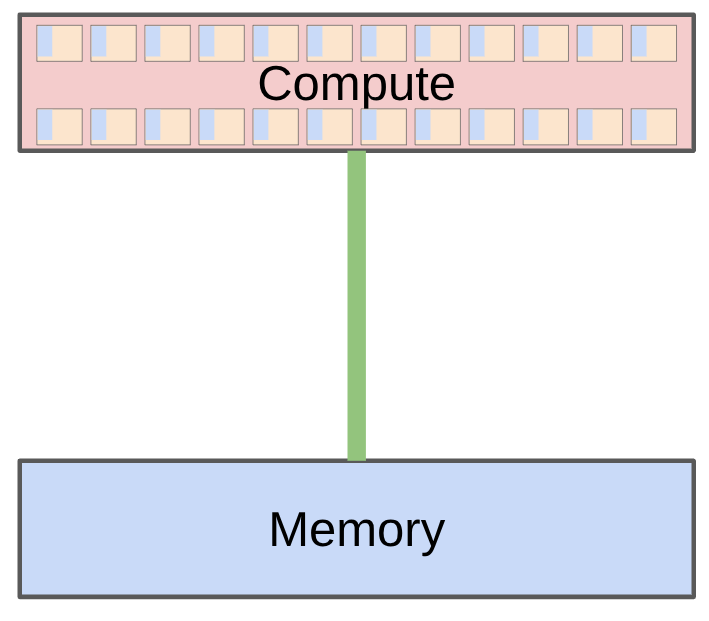
Figure 3.12 Compute and Memory

Percy drew a cartoon diagram to simplify the GPU's working model:

Send inputs from HBM (High Bandwidth Memory) to compute cores
Execute computation
Send outputs from compute cores back to HBM

"You're not just doing a bunch of MatMuls and seeing how long they take. You also have to move data back and forth."

Total time depends on two factors:

Factor	Meaning	H100 Spec
Accelerator speed (FLOP/s)	How fast you can compute	989.5 TFLOPS (bf16)
Memory bandwidth (Bytes/s)	How fast you can move data	3.35 TB/s

"Remember when we cared about memory footprint earlier? Not just because the model is too big to fit in HBM, but because moving data itself takes time. Memory size actually affects speed too."

3.6.2 ReLU Arithmetic Intensity Analysis

Take a simple ReLU operation as an example (1024 × 1024-dimensional bf16 vector):

Memory movement (Bytes):

Read x: 2 × n (bf16 is 2 bytes/element)
Write y: 2 × n
Total: 4n

Compute (FLOPs):

n comparisons (max(x, 0))
Total: n FLOPs

Communication time = 4n / (3.35 × 10¹²) ≈ 1.2 × 10⁻⁶ seconds Compute time = n / (989.5 × 10¹²) ≈ 1.0 × 10⁻⁹ seconds

There's an important assumption here: communication and computation can perfectly overlap. In the ideal case, data arrives and computation begins immediately, while the next batch of data is already in transit. Therefore total time = max(communication time, compute time), not the sum of both.

In this example, communication time far exceeds compute time — ReLU is a classic memory-bound operation.

3.6.3 Defining Arithmetic Intensity

To avoid computing both times and comparing them every time, we introduce Arithmetic Intensity:

Accelerator intensity = FLOP/s / Bytes/s  → H100 is approximately 295 FLOP/byte
Arithmetic intensity = FLOPs / Bytes       → How many FLOPs this operation can do per byte moved

Arithmetic intensity < Accelerator intensity → Memory-bound (bottleneck is data transfer)
Arithmetic intensity > Accelerator intensity → Compute-bound (bottleneck is computation)

"For H100, the accelerator intensity is about 295. This number is worth remembering — for bf16, you need about 300 floating-point operations per byte moved to escape the memory bottleneck."

3.6.4 Arithmetic Intensity Comparison Across Operations

Percy walked through analyzing the arithmetic intensity of several common operations:

Operation	FLOPs	Bytes	Arithmetic Intensity	Bottleneck
ReLU	n	4n	≈ 0.25	Memory-bound
GeLU	20n	4n	≈ 5	Memory-bound
Dot Product	2n-1	4n+2	≈ 0.5	Memory-bound
Matrix-Vector	n(2n-1)	2n²+4n	≈ 1	Memory-bound
Matrix-Matrix	n²(2n-1)	6n²	≈ n/3 ≈ 340	Compute-bound

Key intuitions:

ReLU vs GeLU: Although GeLU's formula contains complex operations like tanh and polynomials, with FLOPs 20× that of ReLU, both take nearly the same time on GPU — because they're both memory-bound, with the bottleneck being data movement, not computation. "You might think GeLU is complex so it must be slow, but it's actually not the bottleneck."
What arithmetic intensity = 0.25 means: Percy said, "If someone tells you an algorithm's arithmetic intensity is 0.25, you should immediately say 'that's terrible.'"
Matrix multiplication's O(n) advantage: For n×n matrix multiplication, you move O(n²) data but do O(n³) computation, so arithmetic intensity is O(n). The larger the matrix, the higher the arithmetic intensity.
Why large batch size matters: "When you're below the accelerator intensity, making the matrix smaller doesn't make it faster — because the bottleneck isn't computation. Only when you exceed the accelerator intensity inflection point are you truly saturating your GPU."

3.6.5 Training vs. Inference Arithmetic Intensity Differences

Percy specifically pointed out:

During training: The input is the entire sequence, equivalent to matrix multiplication. Processing all tokens of a sequence with matrix multiplication has very high arithmetic intensity — it's compute-bound.
During inference: Token-by-token generation, equivalent to matrix-vector multiplication (a vector and a matrix doing dot products). As analyzed earlier, matrix-vector multiplication is memory-bound.

"This explains why inference MFU is far lower than training: you're not feeding the compute units — you're waiting for data to arrive from HBM."

3.6.6 Roofline Plot

Roofline Analysis

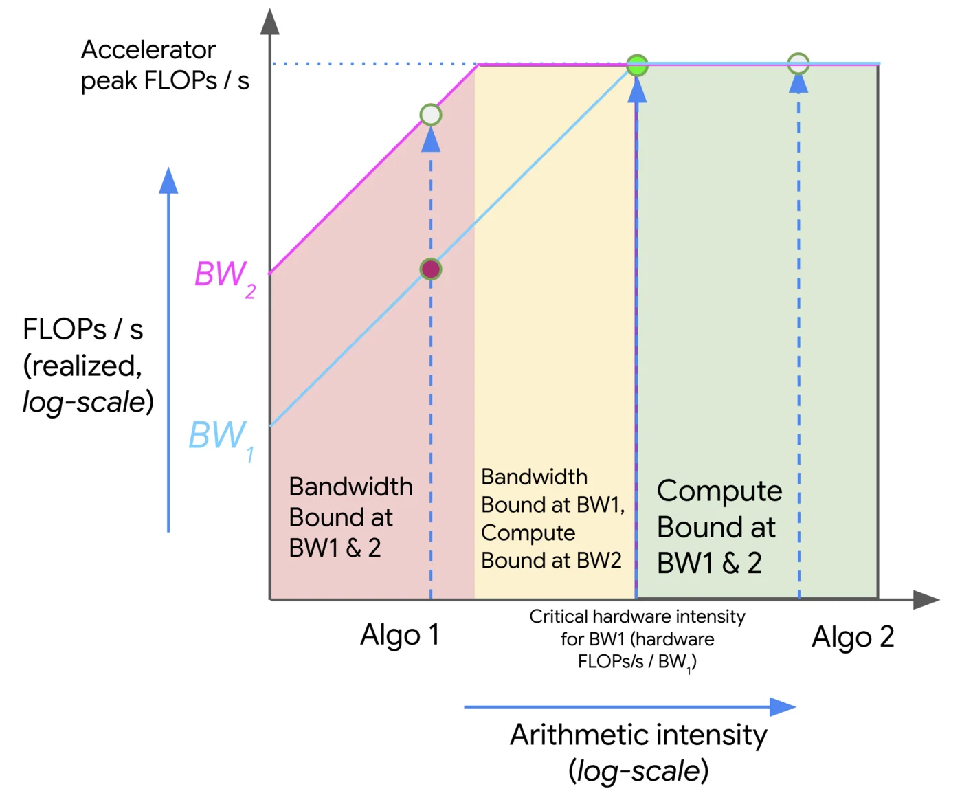
The Roofline plot intuitively shows the relationship between arithmetic intensity and performance:

X-axis: Arithmetic intensity (each "slice" corresponds to a specific algorithm)
Y-axis: Actually achieved FLOP/s
Each piecewise linear curve: A specific hardware platform (H100, B200, etc.)
Inflection point (kink): That hardware's accelerator intensity — left of the inflection point is the memory-bound region (rising slope), right is the compute-bound region (horizontal ceiling)

Percy explained: "If your operation is to the left of the inflection point, it means arithmetic intensity isn't high enough, and actual FLOPs are far below the hardware's peak capability. Only when arithmetic intensity exceeds the inflection point can you approach peak FLOP/s."

Relationship between MFU and Roofline:

MFU = min(1, arithmetic intensity / accelerator intensity)

This is why MFU is typically around 0.5 — many operations have arithmetic intensity below accelerator intensity, causing GPU compute units to "spin idle waiting for data."

A student asked: if most operations are memory-bound, why don't GPUs design better memory bandwidth? Percy answered: "Maybe we can discuss this after you understand more about how GPUs work. If you have a better hardware design, you should tell Jensen (Huang)."

Reference: JAX Scaling Book — Roofline

3.7 Key Takeaways

Learn "napkin math" — quick estimates save months of trial experimentation
Each parameter consumes ~16 bytes during training (param + gradient + AdamW states), plus activation memory
BF16 is the current mainstream — same range as FP32, half the memory, no loss scaling needed
Use jaxtyping + einops for cleaner, less error-prone dimension management
Most view operations (view, transpose, slice) are zero-copy — but non-contiguous tensors need .contiguous()
Minimize CPU↔GPU transfers — PCI bus bandwidth is the bottleneck
Arithmetic intensity determines whether you're compute-bound or memory-bound
Training is typically compute-bound (matrix multiplication), while inference is typically memory-bound (matrix-vector multiplication)

📚 References and Further Reading

DeepSeek V3.2 — DeepSeek V3.2 Technical Report
Mixed Precision Training (2017) — Mixed precision training foundational paper
FP8 Formats for Deep Learning (2022) — FP8 standardization paper
NVFP4 Introduction (2025) — NVIDIA 4-bit floating point introduction
Nemotron 3 Super (2026) — First large model trained in NVFP4
FP8 Primer (NVIDIA) — FP8 getting started guide
Einops Tutorial — Einops official tutorial
H100 Datasheet — NVIDIA H100 specifications
GPT-3 FLOPs Analysis — Lambda Labs analysis of GPT-3 compute
GPT-4 Details Revealed — GPT-4 detail estimates
AdaGrad (2011) — AdaGrad original paper
Transformer Memory Usage (2023) — Transformer memory usage deep dive
Transformer FLOPs — Transformer FLOPs accounting
JAX Scaling Book — Roofline — Roofline analysis reference
PyTorch AMP Documentation — PyTorch automatic mixed precision docs
CS336 Course Website

Chapter 3: PyTorch and Resource Accounting ​

3.1 Why Do We Need Resource Accounting? ​

3.1.1 Scenario 1: Time Estimation ​

3.1.2 Scenario 2: Memory Estimation ​

3.2 Tensors ​

3.2.1 Tensor Basics ​

3.2.2 Tensor Operations ​

Tensor Views ​

Element-wise Operations ​

Matrix Multiplication ​

3.2.3 Optimizing Tensor Operations with Einops ​

1. Naming Dimensions with jaxtyping ​

2. Using einops.einsum Instead of Matrix Multiply + Transpose ​

3. Using einops.reduce Instead of mean(dim=...) ​

4. Using einops.rearrange to Split/Merge Dimensions ​

3.3 Memory ​

3.3.1 Floating-Point Types ​

3.3.2 Tensor Storage Mechanism ​

3.3.3 Moving Tensors from CPU to GPU Memory ​

3.4 Compute Efficiency ​

3.4.1 FLOPs (Floating Point Operations) ​

3.4.2 Arithmetic Intensity ​

3.5 Model Building and Training Fundamentals ​

3.5.1 Parameter Initialization ​

Storing Model Parameters ​

The Importance of Initialization and Common Methods ​

3.5.2 Building Custom Models with PyTorch ​

3.5.3 Managing Randomness for Reproducibility ​

Sources of Randomness ​

Setting Random Seeds ​

3.5.4 Data Loading ​

3.5.5 Optimizer ​

Common Optimizers Overview ​

Using the Optimizer ​

Optimizer Under the Hood ​

3.5.6 Resource Accounting ​

Memory Footprint Analysis ​

Compute (FLOPs) Analysis ​

3.5.7 Training Loop: Integrating All Components ​

3.5.8 Checkpointing ​

Why Do We Need Checkpoints? ​

What Does a Checkpoint Contain? ​

How to Save and Load Checkpoints? ​

Saving a Checkpoint ​

Loading a Checkpoint ​

3.5.9 Mixed Precision Training ​

Mixed Precision Training Overview ​

Tools for Automatic Mixed Precision Training ​

3.6 Arithmetic Intensity and Roofline Analysis ​

3.6.1 Compute Isn't Just About "Computing" ​

3.6.2 ReLU Arithmetic Intensity Analysis ​

3.6.3 Defining Arithmetic Intensity ​

3.6.4 Arithmetic Intensity Comparison Across Operations ​

3.6.5 Training vs. Inference Arithmetic Intensity Differences ​

3.6.6 Roofline Plot ​

3.7 Key Takeaways ​

📚 References and Further Reading ​

Chapter 3: PyTorch and Resource Accounting

3.1 Why Do We Need Resource Accounting?

3.1.1 Scenario 1: Time Estimation

3.1.2 Scenario 2: Memory Estimation

3.2 Tensors

3.2.1 Tensor Basics

3.2.2 Tensor Operations

Tensor Views

Element-wise Operations

Matrix Multiplication

3.2.3 Optimizing Tensor Operations with Einops

1. Naming Dimensions with jaxtyping

2. Using einops.einsum Instead of Matrix Multiply + Transpose

3. Using einops.reduce Instead of mean(dim=...)

4. Using einops.rearrange to Split/Merge Dimensions

3.3 Memory

3.3.1 Floating-Point Types

3.3.2 Tensor Storage Mechanism

3.3.3 Moving Tensors from CPU to GPU Memory

3.4 Compute Efficiency

3.4.1 FLOPs (Floating Point Operations)

3.4.2 Arithmetic Intensity

3.5 Model Building and Training Fundamentals

3.5.1 Parameter Initialization

Storing Model Parameters

The Importance of Initialization and Common Methods

3.5.2 Building Custom Models with PyTorch

3.5.3 Managing Randomness for Reproducibility

Sources of Randomness

Setting Random Seeds

3.5.4 Data Loading

3.5.5 Optimizer

Common Optimizers Overview

Using the Optimizer

Optimizer Under the Hood

3.5.6 Resource Accounting

Memory Footprint Analysis

Compute (FLOPs) Analysis

3.5.7 Training Loop: Integrating All Components

3.5.8 Checkpointing

Why Do We Need Checkpoints?

What Does a Checkpoint Contain?

How to Save and Load Checkpoints?

Saving a Checkpoint

Loading a Checkpoint

3.5.9 Mixed Precision Training

Mixed Precision Training Overview

Tools for Automatic Mixed Precision Training

3.6 Arithmetic Intensity and Roofline Analysis

3.6.1 Compute Isn't Just About "Computing"

3.6.2 ReLU Arithmetic Intensity Analysis

3.6.3 Defining Arithmetic Intensity

3.6.4 Arithmetic Intensity Comparison Across Operations

3.6.5 Training vs. Inference Arithmetic Intensity Differences

3.6.6 Roofline Plot

3.7 Key Takeaways

📚 References and Further Reading