
Chapter 8: Distributed Training
Learning Objectives
Before diving into specific analysis, let's clarify this section's focus. This section covers the core parallel strategies and system implementation for LLM distributed training:
- Understand the necessity of multi-GPU multi-machine parallel architectures, master collective communication operations (All-Reduce, Broadcast, All-Gather, Reduce-Scatter, etc.) principles and cost models
- Deeply analyze core parallel strategies: Data Parallelism (including ZeRO/FSDP memory optimization), Model Parallelism (Pipeline Parallelism and Tensor Parallelism), etc., understanding their communication overhead, memory benefits, and applicable scenarios
- Learn distributed training with PyTorch + NCCL, including collective communication benchmarking and the principles and implementation of Data, Tensor, and Pipeline Parallelism
- Understand GPU hardware interconnect hierarchy (NVLink, NVSwitch, PCIe) and its impact on communication bandwidth
Today's focus will entirely revolve around parallelism across machines. Our goal is to shift from optimizing single-GPU throughput to understanding the complexity and details needed to train ultra-large-scale models. When models grow large, a single GPU can no longer accommodate them, so we need to split models across different machines while fully utilizing all server resources for fast training. We'll face both computational and memory challenges and need to handle heterogeneous communication between different machines. GPUs have different levels of communication methods, which will give rise to multiple parallelization paradigms. In practice, people simultaneously combine multiple parallel strategies. We'll cover the most mainstream approaches one by one, then discuss how to combine them to efficiently train超大 models. Finally, I'll demonstrate through practical cases how these parallel strategies are applied in large-scale distributed training. This chapter is roughly divided into three parts: first introduce networking fundamentals, then analyze how different network hardware corresponds to various parallelization strategies, and finally demonstrate the overall协作 mechanism through case studies.
8.1 LLM Networking Fundamentals
8.1.1 Background on GPU Scaling
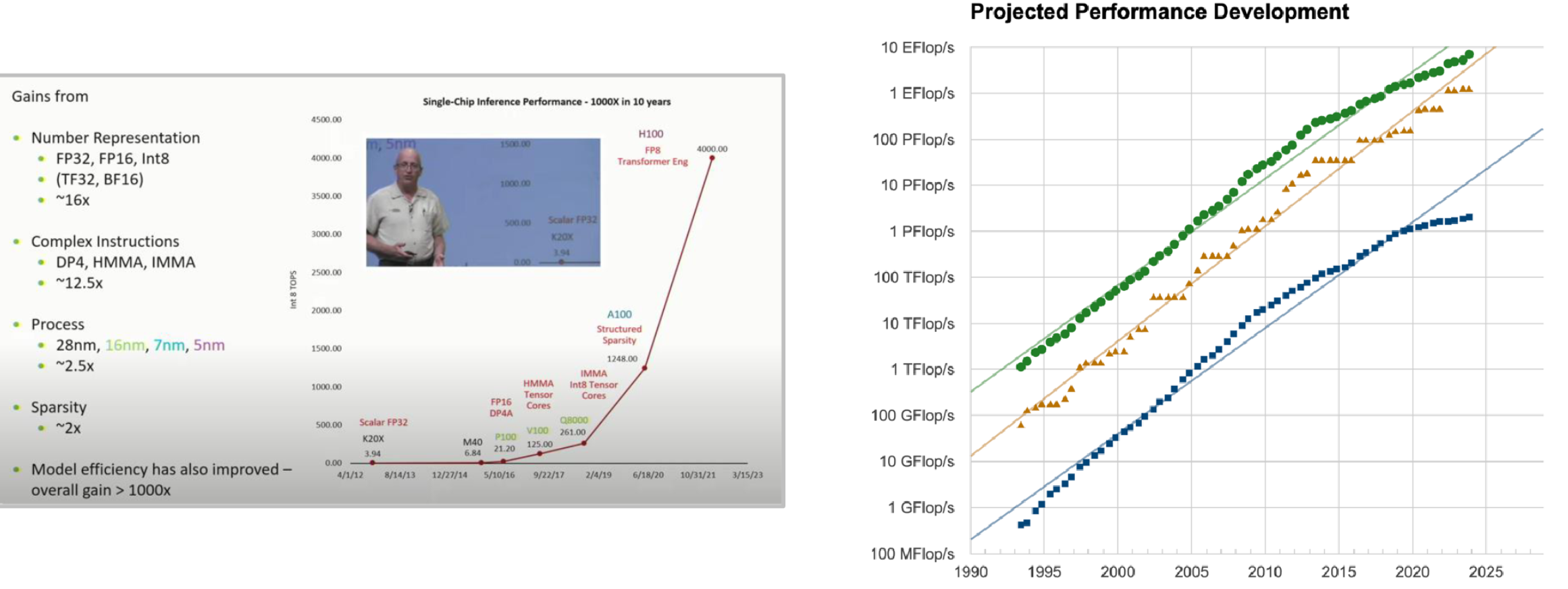
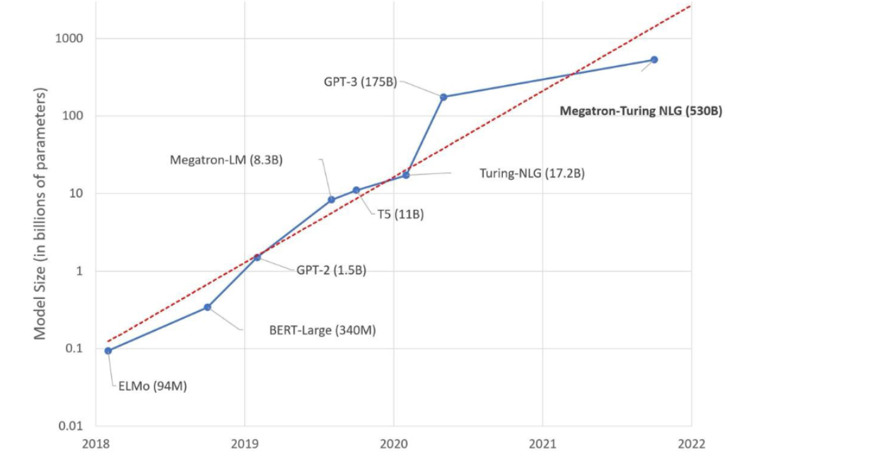
We mentioned GPU compute growth curves in the GPU chapter. Although GPU compute growth is already very fast, relying on a single GPU is insufficient if we want to rapidly scale compute and memory capabilities, because LLM parameter counts are growing extremely rapidly. For example, DeepSeek 671B requires terabyte-level memory, and compute requirements are astronomical — a single card seems utterly inadequate. Although GPU memory is also growing, a single GPU device cannot accommodate such enormous models. The figure below illustrates model size changes (as of 2022).
What we need is a multi-machine parallel architecture — using multiple GPUs to jointly train models. The green curve in the right chart of the first figure represents the world's fastest supercomputers, whose compute power has reached exaflop levels. This is precisely the infrastructure that current cutting-edge LLM training must rely on.
We期望 from multi-machine scaling to achieve linear memory scaling (max model parameters scale with GPU count) and linear compute scaling (model FLOPS scale linearly with GPU count).
8.1.2 Multi-GPU, Multi-Machine Parallel Architecture
So-called multi-GPU, multi-machine parallelism means one machine carries multiple GPUs, with multiple machines computing simultaneously.
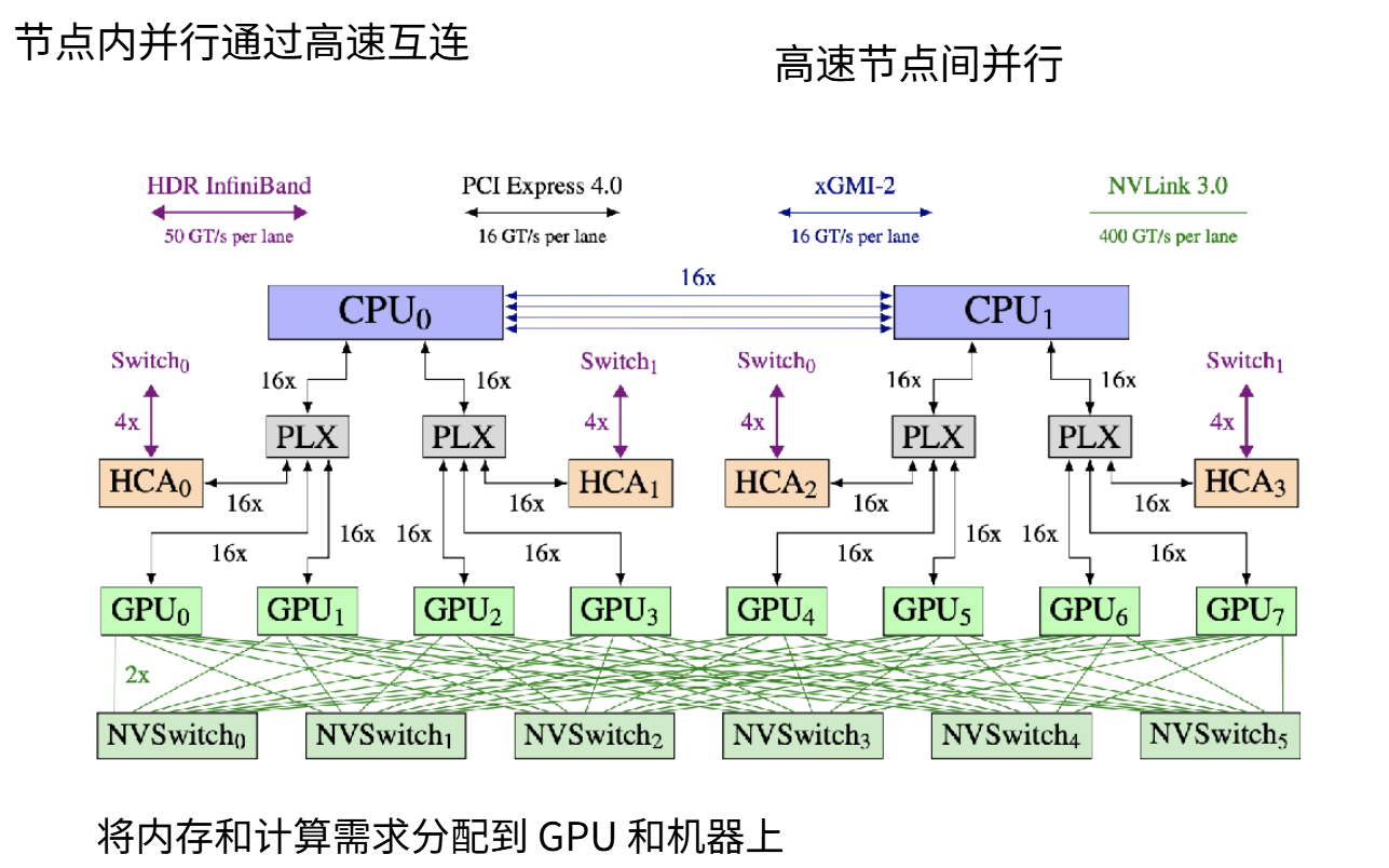
The above is a diagram引用 from the GPTNeoX paper (though the example is older, the principle applies to current H100 machines). One machine has multiple GPUs, with eight GPUs connected to the CPU via high-speed interconnects. At the底 layer, NVSwitch provides extremely fast intra-machine interconnect, but cross-machine communication must go through network switches (shown as purple HDR InfiniBand lines), which is a connection明显 slower than NVLink — data throughput is roughly 8× slower. This hardware hierarchy will directly influence the model parallelization strategies we actually adopt. Remember: intra-machine communication is extremely fast, while cross-machine communication has significant latency.
When we span multiple machines, speed decreases, and depending on the hardware type used, once we exceed (for example) 256 networked GPUs, even more severe slowdowns may occur. Many students who have studied systems or networking courses may already know this, but let's briefly review collective communication operations.
8.1.3 Collective Communication Operations
1. All-Reduce Operation
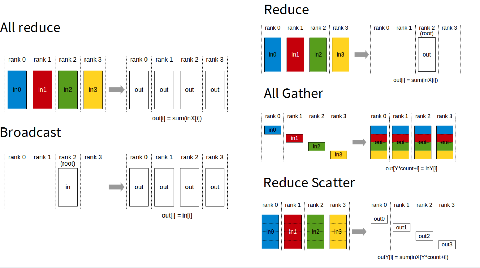
Suppose we have four machines (four nodes), each holding its own data. We need to perform a reduction operation on each node (e.g., summing all inputs), then replicate the four results to every machine. Simply put, the total communication volume of All-Reduce is roughly twice the data volume. Common All-Reduce implementations (like Ring All-Reduce) require
The All-Reduce operation can be equivalently decomposed into Reduce-Scatter + All-Gather. The communication volumes of these two steps also add up to exactly one All-Reduce's communication volume (i.e., 2× parameter count). Understanding this equivalence relationship is very important because it's the theoretical foundation that enables subsequent ZeRO optimizers to achieve "free" memory savings — we can split the originally single-step All-Reduce into two steps, inserting additional computation in between without increasing total communication cost.
2. Broadcast Operation
Taking node 2's single input as an example, replicate it to all other nodes. Communication cost is roughly proportional to the total output volume.
3. Reduce Operation
Sum different inputs (four here) and send them only to one machine.
4. All-Gather Operation
All-Gather means replicating node 0's parameter sub-components to all nodes, with nodes 1/2/3 performing the same operation. Each node processes different parameter partitions and replicates them to other machines. It concatenates all nodes' data chunks and completely replicates them to every node (unlike All-Reduce's "aggregation," All-Gather only does "collection" without "computation").
5. Reduce-Scatter
Reduce-Scatter sums data across rows and sends results only to node 0. That is, first perform reduction computation on all nodes' data, then partition the results so each node only receives its own portion.
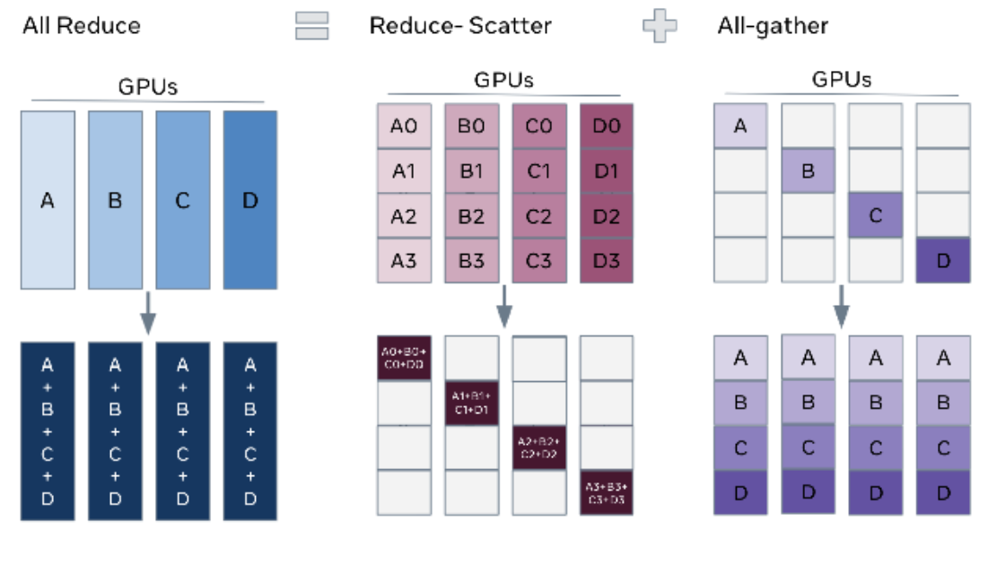
All-Gather and Reduce-Scatter are important because they are essentially the foundational components for building many parallelization algorithms.
For example, when executing All-Reduce: suppose different GPUs (A/B/C/D) process different data points, then we need to sum gradients and send them back to all GPUs — this is a typical four-GPU data parallel operation. But this process can be replaced by two operations: Reduce-Scatter and All-Gather. The former sums across rows and leaves results on GPUs A through D respectively; the latter replicates results to other GPUs. In bandwidth-constrained scenarios, this is the optimal approach. All-Reduce's peak performance is basically equal to the bandwidth limit of Reduce-Scatter plus All-Gather, which can be verified by comparing the communication counts of the two operations.
8.1.4 GPU and TPU
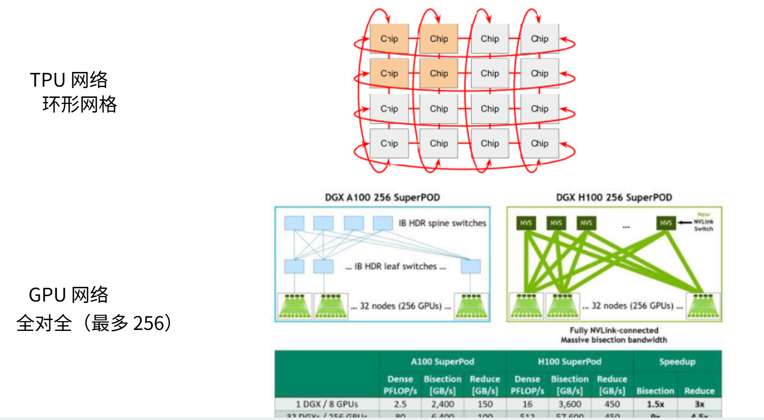
Let's briefly explain the differences between GPU and TPU.
GPU networking is shown in the figure above: a single node contains 8 GPUs, achieving high-speed interconnect through switches, with up to 256 GPUs capable of fully interconnected high-speed communication. Beyond this threshold (roughly one rack's capacity), communication must go through slower switches and spine switches.
Google's TPU uses a fundamentally different networking approach: a single TPU chip achieves extreme-speed communication with adjacent nodes, forming an easily scalable torus mesh structure, but only supports adjacent-node communication.
We discuss this immediately after All-Reduce because on a torus mesh, the efficiency of collective communication (like All-Reduce or Reduce-Scatter) is comparable to fully interconnected solutions. If purely optimized for collective communication, TPU network architecture has advantages over GPU networks. Later, we'll discuss a data center rather than a single GPU.
Fat Tree vs. Torus Mesh Differences
GPU interconnect uses "fat tree" topology: within nodes, full interconnect via NVSwitch; between nodes, extension via spine switch, suitable for random, unpredictable communication patterns (like MoE). TPU uses a 3D torus mesh — each chip only communicates with neighbors, boundaries wrap around, topology is極简, and it's extremely efficient for dense collective communication.
The two are undergoing convergent evolution: Google's next-generation TPU (Trillium) has already shifted to tree topology to support the all-to-all communication needed by MoE. This shows that model workloads are反过来 defining the required network topology.
Extreme Hardware Trade-off: Huawei Ascend 910
Huawei Ascend 910's single-chip compute is far weaker than H200, but through fiber optic switches, 384 chips are fully interconnected, using brute-force scaling to compensate for single-chip compute insufficiency. The cost: power consumption reaches 4× that of equivalent NVIDIA systems. This embodies the extreme engineering trade-off of "trading power for communication," similar in logic to Groq building chips entirely from SRAM.
8.2 Core Parallel Strategies
We need to focus on three parallel strategies.
First is Data Parallelism — its core idea is replicating parameter copies across different GPUs, not involving parameter splitting, but partitioning the training batch so different GPUs or machines process different slices of the data batch — this is data parallelism.
Second is Model Parallelism. As model scale grows, one GPU can hardly fit all model parameters. Therefore, we need to partition the model so different GPUs handle different parts of the model.
Finally is Activation Parallelism. In daily development, we rarely关注 activations because PyTorch handles them transparently. But as model scale and sequence length grow, activation memory becomes a severe challenge. To train giant models with ultra-large batches, we must effectively manage activation memory footprint, hence activations also need to be partitioned.
When these three parallel strategies work协同, we gain the ability to elegantly scale computation across vast machine clusters.
8.2.1 Data Parallelism
The core idea: replicate model, shard data batches.
Data parallelism starts from the most朴素 stochastic gradient descent (SGD).
Where:
As shown in the formula, we take batch size B, accumulate all gradients, then update parameters. The most basic data parallelism partitions batch B across different machines, with each machine computing partial gradient sums. Then before each gradient update, synchronize all gradients — specifically, first exchange all gradients for synchronization, then execute parameter update.
Data parallelism is very effective. Each machine's GPU receives B/M samples. When the batch size is sufficiently large, each GPU gets reasonably sized batch data and can fully saturate compute resources. However, each batch requires transmitting twice the parameter count in data, because the communication cost of all-reduce approximately equals twice the data volume being reduced. When batch sizes are large, this overhead is acceptable because the communication cost of频繁 gradient synchronization can be hidden.
But the current approach完全没有 optimize memory. Each GPU needs a complete copy of parameters and optimizer states, which is extremely不利 for memory scaling. In actual training, memory is always the bottleneck — we've all encountered PyTorch OOM errors when loading large models onto GPUs. This directly impacts training effectiveness, so ideally we need to save memory.
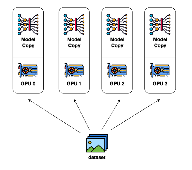
In naive data parallel memory usage, we need to store many model copies. Depending on training precision, each parameter requires approximately 16 bytes of storage — in practice, we need to保存 about 5 weight copies.
From the model parameter perspective alone, storing FP or BF16 theoretically requires only 2 bytes. We also need to store gradients (another 2 bytes at BF16 precision), optimizer states: SGD cumulative updates need 4 bytes master weights, Adam first-moment estimates need 4 (or 2) bytes (for recording historical gradients), second-moment estimates (gradient variance) need another 4 (or 2) bytes.
ZeRO Solves DP (Data Parallelism) Memory Overhead
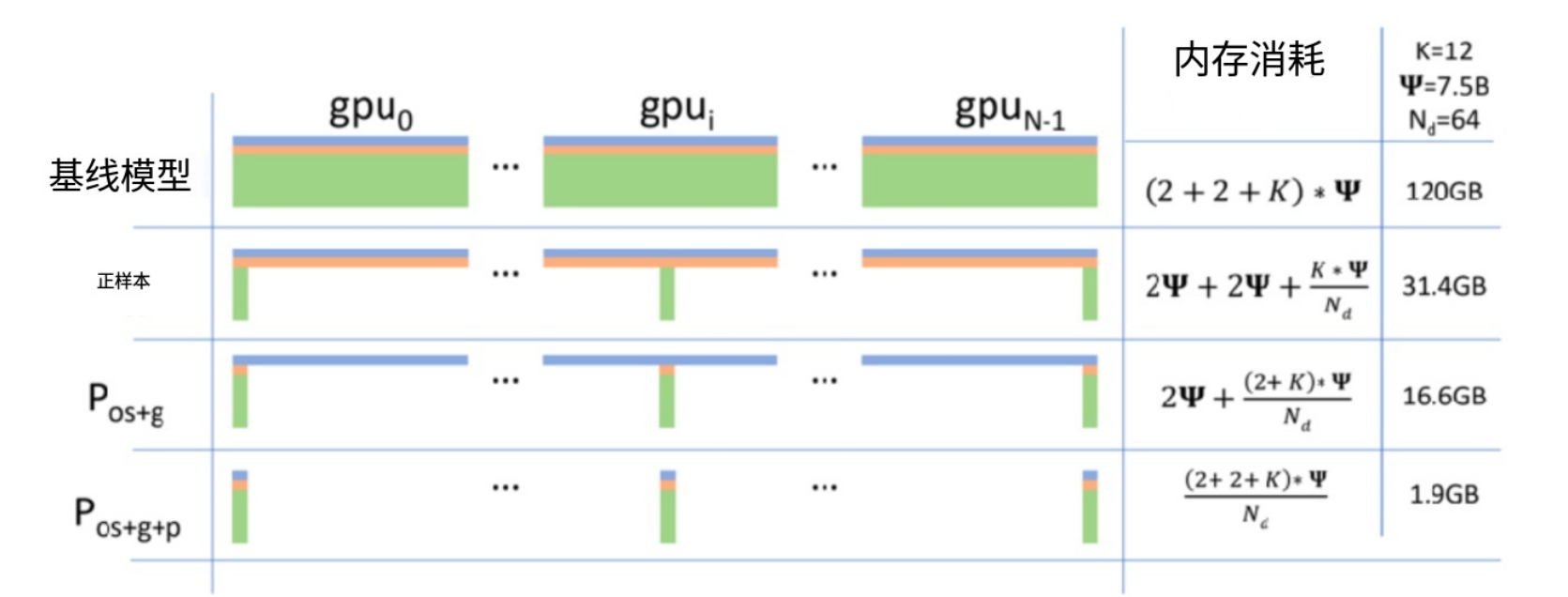
Blue portion is parameter memory, orange is gradients, green is optimizer state memory
Through the diagram, we can直观 see that in parameter memory footprint, Adam optimizer state occupies the majority, so memory consumption mainly depends on optimizer state byte count — typically even exceeding core parameter and gradient memory usage.
Taking a 7.5B parameter model distributed across 64 accelerators as an example, its memory footprint is极其庞大, and total memory grows linearly with GPU count — this is clearly unacceptable.
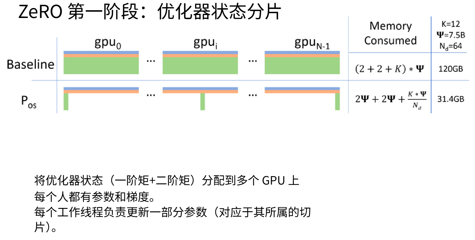
Parameter and gradient跨-device replication is a necessary part of data parallelism, but all optimizer states don't need to exist on every machine — i.e., optimizer state sharding. From the figure above, we can see that through this technique, total memory footprint can drop from 120 GB to 31.4 GB. If we further shard gradients, memory usage can compress to 16.6 GB. When parameters are also sharded, memory footprint can ultimately be optimized to 1.9 GB. This would be a相当 ideal state, because now we've completely sharded all needed optimizer states, parameters, and gradient memory.
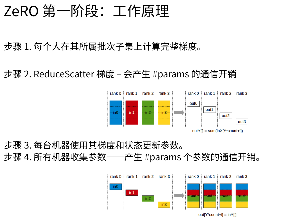
Step 1: Suppose each GPU gets different data points. Suppose GPUs 0 through 4, each GPU processes a single sample and computes complete gradients based on its own sample.
Step 2: Execute gradient Reduce-Scatter operation, collecting gradients held by each GPU. Suppose GPU0 is responsible for the first quarter of parameters. Through Reduce-Scatter, ensure GPU0 obtains all gradient information from all other GPUs for its responsible parameter subset. Thus, it汇集了 gradient information from GPUs 1/2/3, all reduced onto GPU0. Now GPU0 possesses all information needed to update its own parameters, holds the optimizer states corresponding to the first portion of parameters, and also possesses the complete aggregated gradients for that portion.
Step 3: Use gradients and states to perform gradient update on this portion of parameters.
Step 4: GPU0 now has the fully updated version of this parameter subset. Finally,只需 through an All-Gather operation, synchronize all updated parameters back to all compute nodes.
The key here is we're doing Reduce-Scatter and All-Gather. Reduce-Scatter plus All-Gather costs the same as All-Reduce. We previously did All-Reduce on all gradients to ensure everyone's gradients were synchronized, which cost 2× our parameter count. We can perform some computation between the Reduce-Scatter and All-Gather steps. This gives us the same compute-communication cost but more computation operations.
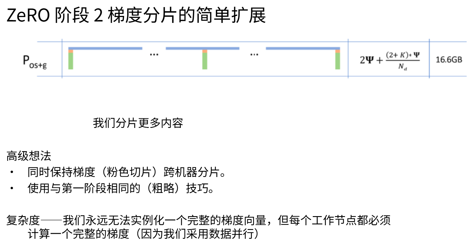
Next, further expand the sharding scope to include gradients. Complete parameters + sharded gradients + sharded optimizer states.
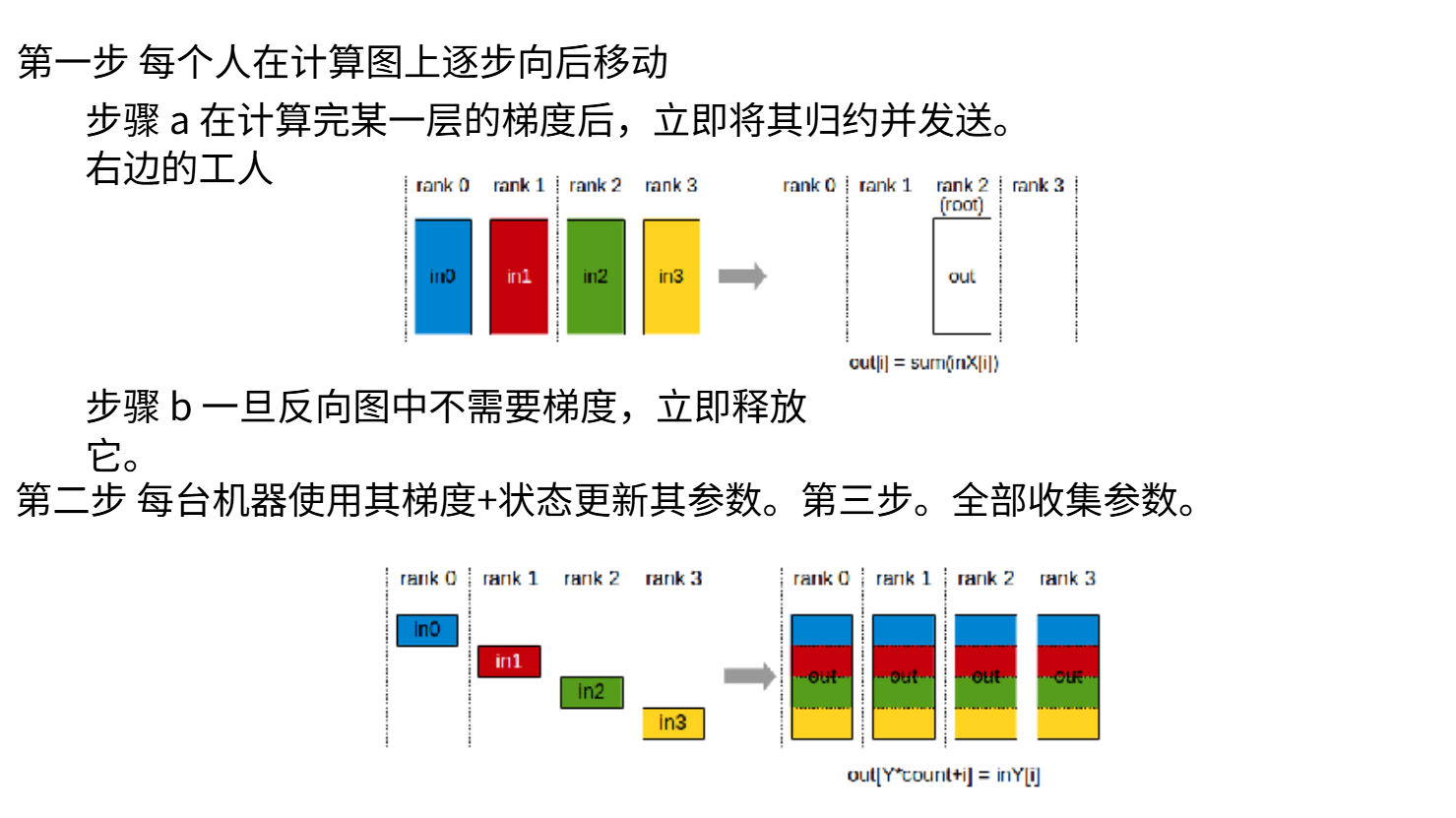
The specific process: during backward gradient computation, whenever a certain layer's gradient computation completes, immediately send it to the corresponding GPU. All compute nodes each hold batch data components, computing backward along the computation graph step by step. Suppose we operate by layer (each layer atomically sharded to different GPUs), then after completing each layer's gradient computation in the backward computation graph, immediately invoke reduction operation to send gradients to the corresponding worker node. For example, if a certain layer belongs to GPU 2, we immediately execute reduction operation and send to that node. At this point, gradient data no longer needs to be retained, so we don't need to store gradients on compute nodes 0, 1, 3 — they can be immediately released from memory. The reason: a single GPU cannot cumulatively保存 all gradients.
This cycle repeats, and ultimately all machines obtain fully updated gradients. Now each machine holds complete gradients for its corresponding parameter分量, also holds complete optimizer states for its corresponding parameter分量. Each updates its own parameters, then整合 parameters via All-Gather. Although it appears communication volume increases (because each layer requires reduction operations), this only involves small parameter counts (since they're already sharded), so total communication volume remains unchanged. ZeRO Stage 2 does introduce additional overhead (needing逐层 synchronization to ensure correct gradient delivery), but the overhead is very limited, and the overall implementation remains简洁直观.
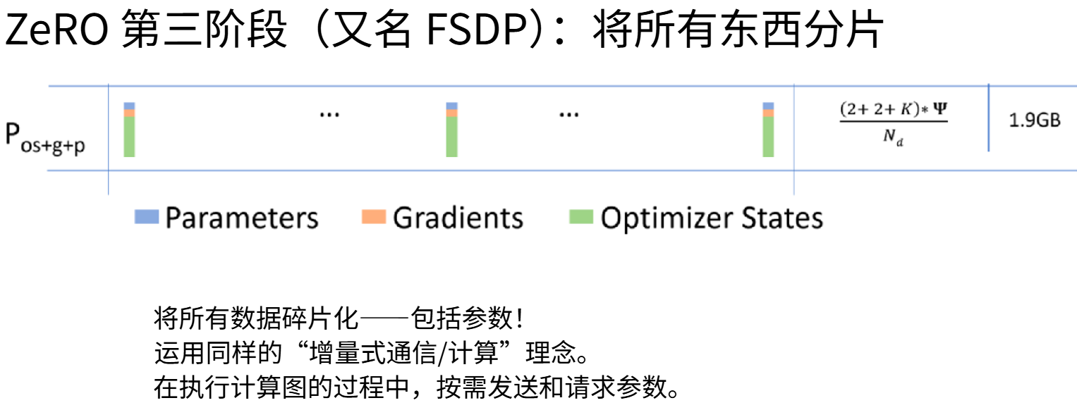
Finally, ZeRO Stage 3 — more complex but with greater benefits. Now all components (including parameters) can be evenly divided according to GPU count, achieving maximum memory savings. FSDP (Fully Sharded Data Parallelism) is essentially the concrete implementation of ZeRO Stage 3.
The core idea is to shard all components (including parameters),沿用 ZeRO Stage 2's incremental communication-computation strategy, avoiding保存庞大 gradient vectors. When traversing the computation graph (including forward and backward propagation), send and request parameters on demand. The key is minimizing overhead as much as possible.
FSDP's most amazing feature is achieving this with relatively low overhead.
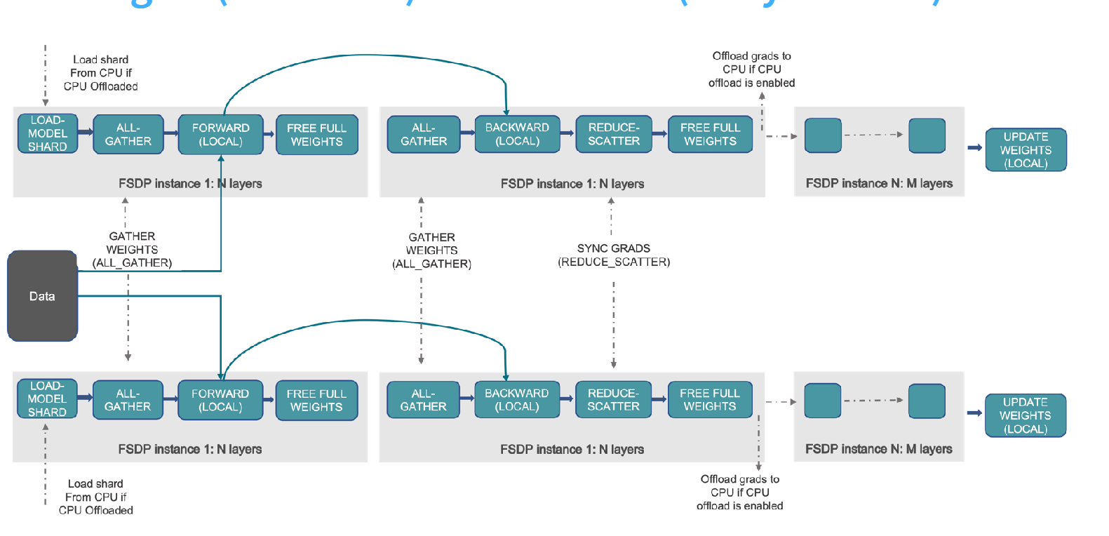
The figure above reveals the overhead control principle. We dynamically整合 model weights through All-Gather operations. For each layer, no single GPU possesses all parameters. Unlike conventional approaches where GPU0 directly executes forward propagation — suppose GPU0 only holds the bottom-layer parameters. After completing that layer's computation, it pauses and requests parameters from all other worker nodes. At this point, it pauses and executes an All-Gather operation (the all-gather step labeled in the figure), obtaining the data needed for forward propagation by汇集 all parameters. It can then continue forward computation for layers it originally lacked, immediately releasing weight data after completion. Then continue All-Gathering the next layer's parameters, executing forward propagation and releasing weights, cycling repeatedly. But activations must be retained, causing activation memory to continuously grow — this eventually becomes a problem.
If we暫不考虑 activations, this pattern is very ideal: load single-layer parameters, execute forward propagation, immediately release — memory overhead is极低. After completing forward propagation, backward propagation follows the same logic: each time computing backward in the neural network, All-Gather the needed parameters, update computed gradients via Reduce-Scatter, then release weights. Ultimately, we can release both unneeded gradient data and parameters, obtaining a fully updated model.
Three core operations need attention here: two All-Gathers and one Reduce-Scatter — essentially completing model synchronization after gradient update. Conceptually, this is just one more operation than ZeRO Stage 2, but does bring more overhead. Total communication cost is now higher: previously 2× parameter count communication volume, which was某种程度上 zero-cost; now reaching 3× parameter count communication cost, plus needing to bear additional overhead from communication waiting.
FSDP's most exquisite aspect is its unexpectedly低 overhead. Despite needing to continuously request and transfer parameters — you might think this causes severe latency — through the core design of overlapping communication and computation, GPU can continuously work while communicating in the background, similar to a prefetch mechanism. When certain data is needed, it's already been transferred and ready.
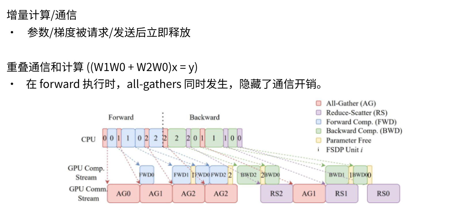
As shown above:
Now observe the communication and computation timing on the device. When computing layer 1, the communication unit has already prefetched layer 2 parameters; when computing layer 2, the communication unit has prefetched layer 3 parameters, forming a pipeline operation. This design allows communication to be almost completely hidden. Although theoretically requiring 3× communication volume, actual efficiency loss may only be 10%-20%.
So at the very beginning, we must ensure every device possesses layer 0's weights, i.e.,
This process is very rapid. Before needed, forward computation 2's required parameters have already been preloaded and completed, so there's no idle period here. Then we can release the second set of parameters.至此, the complete forward propagation process ends. We can see the gaps here are relatively small — we completed大量 loading operations before actual computation occurred. Through this clever preload weight request queue mechanism, we can avoid大量通信 overhead. When forward computation 2 completes, forward propagation is entirely finished. I can release the second set of weights and begin backward propagation. We can see the all-gather 2 operation needed for backward propagation was already completed long ago, so we can immediately start backward computation 2 and backward computation 0, with weight 0 already stored and ready.
The backward propagation phase will exhibit higher overhead because it requires operations like Reduce-Scatter and All-Gather. Although we adopted this extreme sharding strategy (recalling the earlier diagram — we fully sharded parameters, gradients, and optimizer states), the total bandwidth needed is only 3× rather than 2× — this is还算不错. The actual gaps are not severe — communication resources are几乎完全 utilized, and computation stall time is very short. This shows we're实际上 very efficiently utilizing available resources.
Regarding where preloaded weights are stored: Since GPU memory is full, where are these weights preloaded to? We need a buffer to store these weights. Reading current-layer weights incurs some overhead. Another important factor: we completely didn't discuss activations, and this portion occupies很大 space because the entire model's activation collection某种程度上 needs to persist continuously.
Data parallelism's communication cost: 2× parameter count communication.
ZeRO Analysis
From a certain perspective, ZeRO's approach is how people efficiently implement distributed data parallelism. Stage 1 is basically zero-cost — it adopts the same communication pattern as naive data parallelism but can also shard optimizer states. ZeRO Stage 2's communication parameter count is twice the original, so total bandwidth consumption is the same, but gradually releasing gradients during backward propagation brings additional overhead. ZeRO Stage 3 is more complex — program communication cost reaches 3×, but actual performance is不错. The diagrams we saw earlier确实 show some overhead, but if communication patterns are cleverly designed, the results are actually相当理想. Therefore, even with slower network connections, people still use this type of data parallelism. Another advantage of this method: data parallelism has几乎 no special architecture requirements. All details are highly abstracted, which also explains why FSDP is so popular — just write a wrapper to parallelize any neural network without deeply understanding the architecture's specific operational mechanisms.
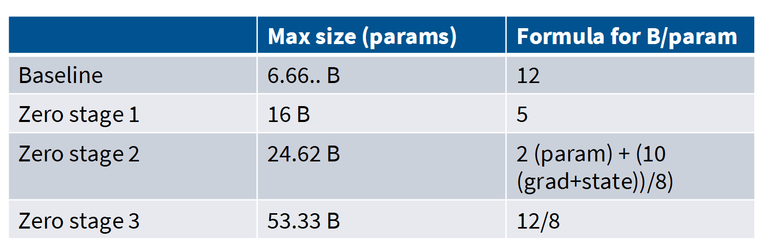
Here are some concrete cases. We can see the maximum model size that can be accommodated on an 8×A100 80GB node. The baseline barely fits a 6B parameter model, while using ZeRO Stage 3 can accommodate approximately a 50B parameter model. Through intelligent memory optimization techniques like FSDP, we gain显著 capability improvement for hosting larger models.
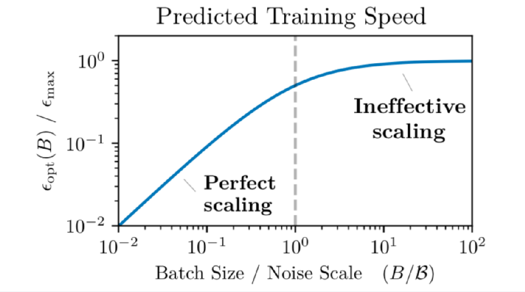
Finally, emphasize the key to data parallelism: batch size is the core limiting factor. Since each machine processes at most one sample instance, data parallelism degree cannot exceed batch size. When batch size reaches its upper limit, data parallelism cannot continue scaling. Everyone may notice that when batch size exceeds a certain critical point, optimization returns show明显的 diminishing returns. Many papers have been published on this topic. OpenAI has an excellent paper discussing critical batch size — their基本观点 is that beyond a certain critical point, each training sample's contribution to optimization capability shows steep diminishing returns. Intuitive understanding: below a certain batch size, gradient noise is large, so reducing noise is very beneficial; but reaching a certain point, the fundamental limiting factor becomes gradient update count rather than variance reduction. This means pure data parallelism cannot achieve arbitrary-scale parallelization — batch size is a very important resource. Essentially, we have a fixed maximum batch size ceiling but can allocate usage in different ways, because other types of parallelization同样 benefit from larger batch sizes. We need to reasonably allocate batch size at specific stages. Data parallelism still has inherent limitations: ZeRO Stage 1/2 cannot scale memory, Stage 3 is theoretically不错 but runs slowly. More importantly, related to the earlier issue, it cannot reduce activation memory.
The most ideal scenario is to completely partition the model into independent parts, so activation memory will also decrease accordingly. Therefore, we need better model partitioning strategies to fit ultra-large-scale models into GPU memory. This brings us to Model Parallelism. Our goal: expand memory capacity while keeping batch size unchanged, and find new dimensions that don't require large batches for parallelization. The specific implementation distributes parameters across multiple GPUs — somewhat similar to ZeRO-3, but instead of passing parameters, we pass activations. This creates critical differences because sometimes activations are much smaller than parameters, which is very有利 for us.
Fundamental Limitation of Data Parallelism: Critical Batch Size
Data parallelism consumes a key resource — global batch size. If global batch size is 8, data parallelism degree can at most reach 8 and cannot scale further.
Even if we强行 increase batch size, there exists the Critical Batch Size limitation: when batch size exceeds a certain threshold, each新增 sample's optimization contribution急剧递减. Because at this point, the model performance constraint has shifted from "gradient noise" to "gradient update steps" — continuing to increase batch size is not equivalent to adding more SGD steps.
Therefore, batch size is a finite resource that needs to be shared among multiple parallel strategies and cannot be arbitrarily allocated to data parallelism.
8.2.2 Model Parallelism
The core idea of model parallelism is distributing parameters across multiple GPUs, similar to ZeRO-3, but what's communicated is activations rather than parameters.
We'll introduce two types of model parallelism: Pipeline Parallelism — conceptually simple but complex to implement; Tensor Parallelism — conceptually more subtle but more elegant in implementation and more widely applied. They correspond to two different model partitioning approaches.
1. Pipeline Parallelism
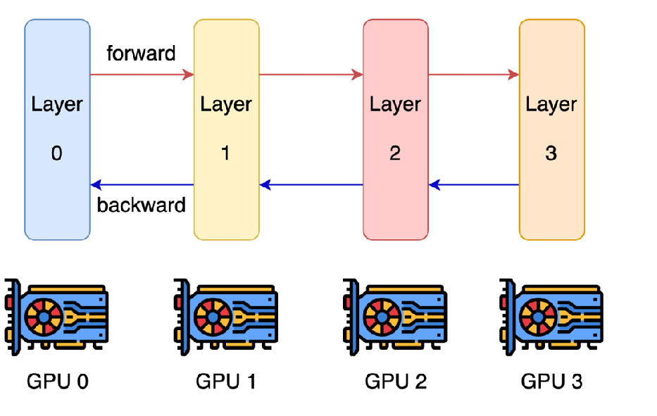
Pipeline Parallelism is perhaps the most intuitive way to partition neural networks. Deep neural networks consist of many layers, so it's natural to think of cutting along layer boundaries — each GPU handles a subset of layers, communicating by passing activations. In this case, each layer is专属 to one GPU. GPUs forward-pass activations to each other, and during backward propagation, gradients are passed back from GPU 3 toward GPU 0. This方案 appears perfect, but the problem is that most GPUs spend most of their time idle — utilization is extremely low because it's layer-by-layer: before the previous layer's activations are computed, all GPUs for subsequent layers are waiting.
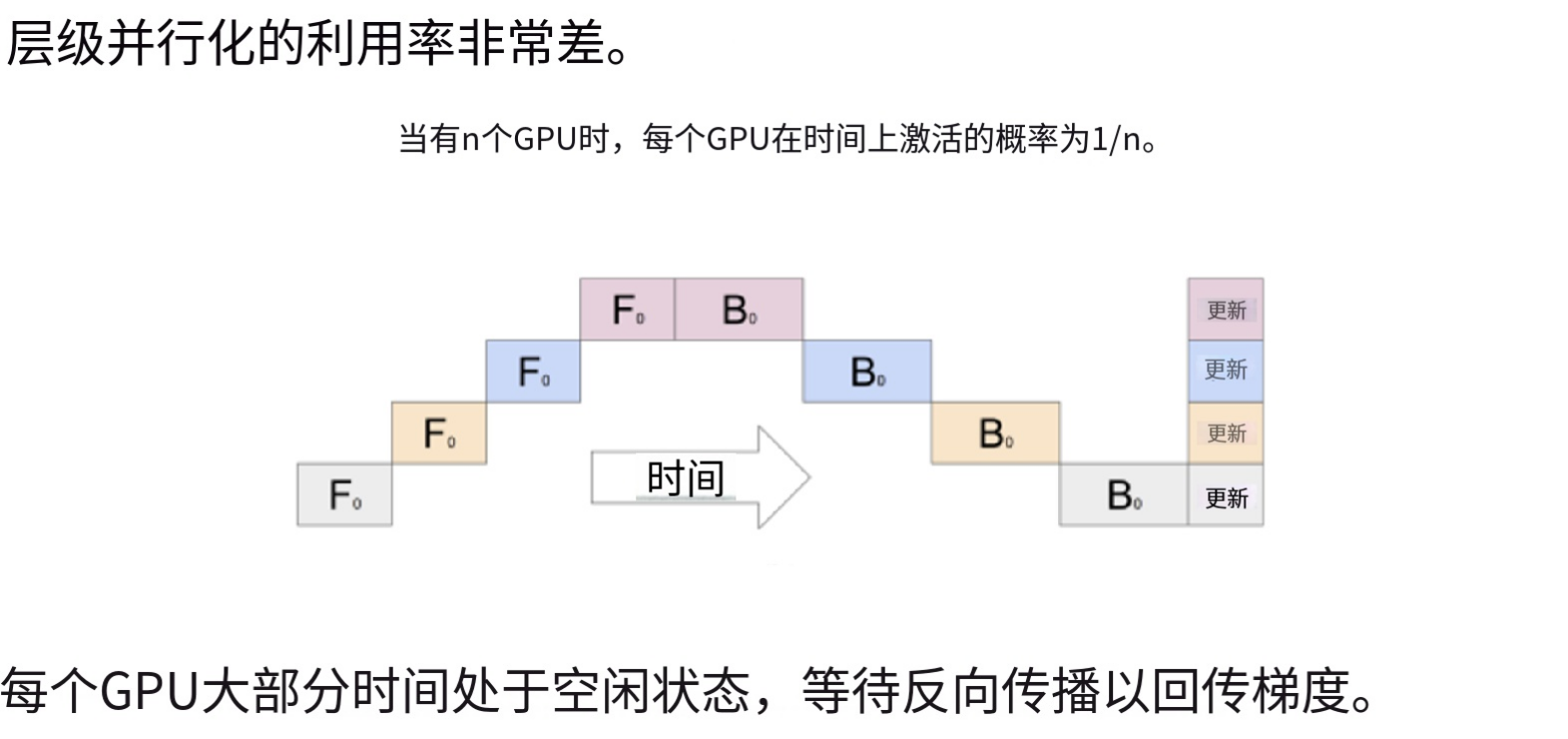
If we adopt this naive parallel approach: suppose each layer包含 forward computation and only processes a single sample, the timeline diagram will呈现 this scene — different rows in the above figure represent different layers (corresponding to different GPUs), with the horizontal axis being the time dimension. We can see the leftmost first computes layer 1, activations propagate to layer 2, then GPU 2 begins working, and so on. By the time backward propagation starts, there's a巨大的 "bubble" — this blank period完全没有 computation, and GPU effective working time is only 1/n. So in a sense, this may be the worst possible parallel方案 — although 4 GPUs were added, the throughput obtained is comparable to a single GPU.
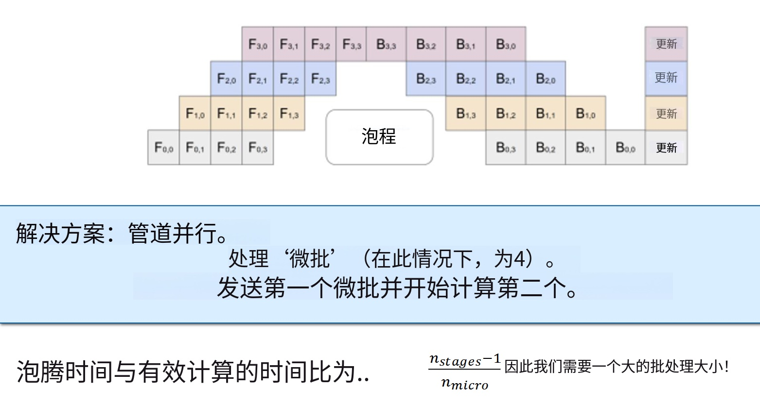
Therefore, we can adopt a more clever approach: build a pipeline architecture. Instead of simply splitting tasks by layer, create task sequences that require each GPU to process in order. Suppose we now have micro-batches, with each machine processing four samples. After completing the first data point's processing, we can immediately send its activations to the second GPU, then immediately begin processing the second data point. This achieves overlap of communication and computation — while the first GPU continues working, the second GPU can also begin working. By increasing batch size, we can effectively shrink the idle periods (bubbles) in the pipeline. This also explains why we earlier referred to batch size as a resource: during pipeline parallelism with fixed batch size, we can either use it to shrink pipeline bubbles or for data parallelism. A single batch size can be partitioned in multiple ways. Micro-batch size actually controls bubble duration. Specifically, the ratio of system overhead to effective computation equals (pipeline stage count)^(-1) divided by micro-batch count. When batch size is sufficiently large, pipeline parallelism can potentially operate efficiently. But as noted earlier, batch size has an upper limit and cannot be arbitrarily expanded.
Although Pipeline Parallelism (PP) is typically lower in parallel efficiency than DP and TP — for example, introducing "bubbles" due to inter-stage dependencies that reduce device utilization — it is still widely adopted in practical systems, primarily due to its trade-off between memory and communication:
- In terms of memory, PP partitions the model by layer across different devices, so each device only needs to store its所属 stage's parameters and activations, effectively reducing per-device memory pressure. This complements parameter sharding methods like DeepSpeed ZeRO: the latter primarily shards parameters and optimizer states, while PP reduces activation storage requirements through structural partitioning;
- In communication patterns, PP only performs point-to-point partial activation transfers between adjacent stages, avoiding the large-scale All-Reduce global synchronization communication typical of DP and TP. Therefore, in cross-node or even cross-card scenarios where global communication bandwidth is constrained or latency is high, PP often has better scalability;
For TPUs (like Google TPU v4) using high-bandwidth ring/mesh interconnects, All-Reduce and cross-device communication in large clusters become more efficient, thus favoring DP and TP efficient scaling in practice. However, parallel strategy selection depends not only on model scale and memory constraints but is also significantly influenced by communication overhead (bandwidth and latency). PP is primarily used to partition models when a single device or tensor parallelism cannot accommodate the model, with its communication pattern being point-to-point transfers between adjacent stages, relatively insensitive to network topology (applicable across both TPU and GPU architectures).
In large-scale training systems like TPU and GPU clusters, although GPU cluster interconnect bandwidth is typically lower than TPU Pods, PP is usually adopted as a supplementary方案, combined with DP and TP. For example, within nodes, high-speed interconnects primarily execute TP, while between nodes, PP reduces cross-node global communication overhead, thereby balancing memory, communication, and parallel efficiency. In contrast, PP partitions the model by layer into multiple stages and executes in a pipelined manner, with sequential dependencies between different stages limiting overall parallelism — the "bubble" phenomenon is precisely the manifestation of these stage dependencies during execution.
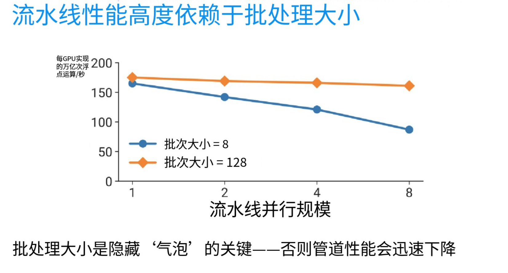
The above figure is an example from an NVIDIA paper: when batch size is 8, as the number of pipeline-parallel devices increases, per-GPU utilization sharply drops; whereas when batch size reaches 128, even with relatively large-scale pipeline parallelism, high utilization can still be maintained. This shows that batch size is crucial for hiding bubble duration.
Of course, we can also adopt more advanced pipeline scheduling strategies — by subdividing the computation graph into finer-grained stages, assigning different sublayers to different devices, and executing different computations at different time periods, thereby achieving better pipeline interleaving.
Zero-Bubble Pipeline Principle
Particularly worth关注 is zero-bubble pipeline technology (called dual pipeline in DeepSpeed). Its core technique: during backward propagation gradient computation, decompose it into two components — one is backpropagating activations along residual connections, i.e., computing derivatives with respect to activations; the other is computing weight gradients.
1F1B Scheduling Strategy (One Forward, One Backward)
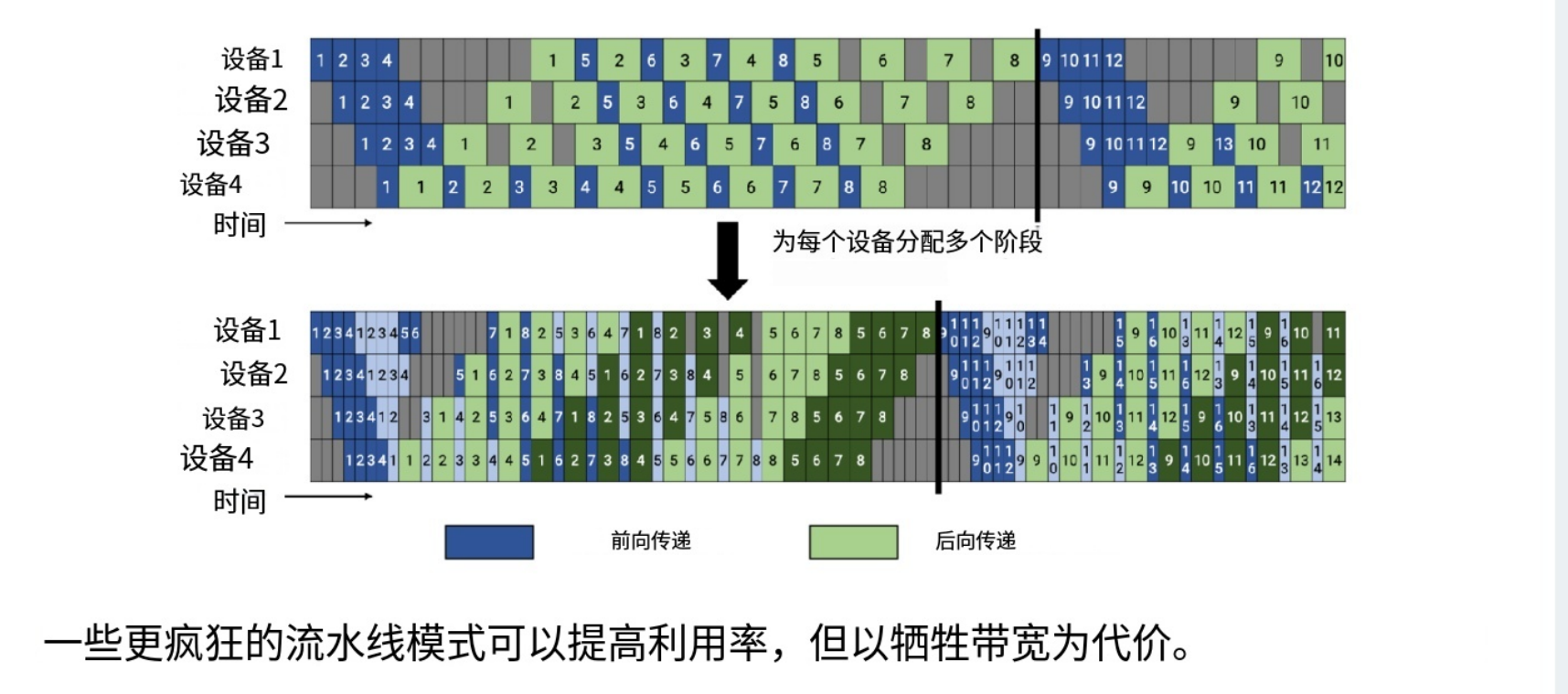
1F1B is one of the most classic scheduling strategies in pipeline parallelism, proposed by NVIDIA in Megatron-LM, specifically designed to address two fatal flaws of naive pipeline parallelism (like GPipe): activation memory growing linearly with micro-batch count and excessive pipeline bubbles.
In GPipe scheduling, a device must first complete all micro-batches' forward propagation before beginning backward propagation. This brings two serious problems:
Backward propagation requires intermediate activations from forward computation. Only after all forwards complete does backward start, meaning all micro-batches' activations must be continuously preserved in memory. With
1F1B's core idea is to change execution order, alternating forward and backward computation. Its key insight: the earlier backward propagation starts, the earlier its needed forward activations can be released, thereby simultaneously compressing memory footprint and bubble time.
Three-Phase Execution Process
Assume
Warmup Phase The device first performs several consecutive forward computations to "fill" the pipeline with micro-batches. Device
performs forwards first. For example, the last device ( ) has no warmup and directly enters steady state; the first device ( ) needs warmup forwards. Steady Phase After reaching stability, the device enters a rhythm of "do one forward, immediately followed by one backward." Each time a new micro-batch's forward completes, immediately take one cached forward result for backward computation. Thus, each new activation produced consumes one old activation and releases its memory. The number of activations simultaneously resident on the device remains constant, no longer growing with
, thereby solving GPipe's memory explosion problem. Cooldown Phase After all forward tasks complete, the device only executes remaining backward propagation until the pipeline empties.
Memory Savings Effect
In GPipe, each device must store
Bubbles Compressed but Still Exist
1F1B compresses bubbles from GPipe's "entire forward phase + entire backward phase" into fixed small bubbles at the pipeline's beginning and end. However, since forward and backward computation times are typically asymmetric (forward time is usually shorter than backward), constrained by the fixed alternating rhythm, bubbles cannot be completely eliminated. This is precisely the direction that subsequent zero-bubble technology continues to optimize — by splitting backward into B (gradient propagation) and W (weight gradient computation), deferrable W computations can fill these residual bubbles.
Going Further
Traditional pipeline scheduling, even with 1F1B, still has bubbles. A further approach splits backward propagation into two parts:
B (Backward): Compute the derivative of loss with respect to activations and propagate toward lower layers along the computation graph. This step has strict sequential dependencies and must execute in order. W (Weight gradient): Compute gradients of current-layer weights. This is leaf-node computation with no downstream dependencies — can be done at any time. Therefore, we can prioritize快速 completing all B computations while deferring W computations to idle periods where bubbles would原本 occur. Through this fine-grained scheduling, pipeline bubbles can be almost completely filled, achieving near-zero idle utilization. DeepSpeed's "dual pipeline" is based on this idea, but its implementation is极其 complex.
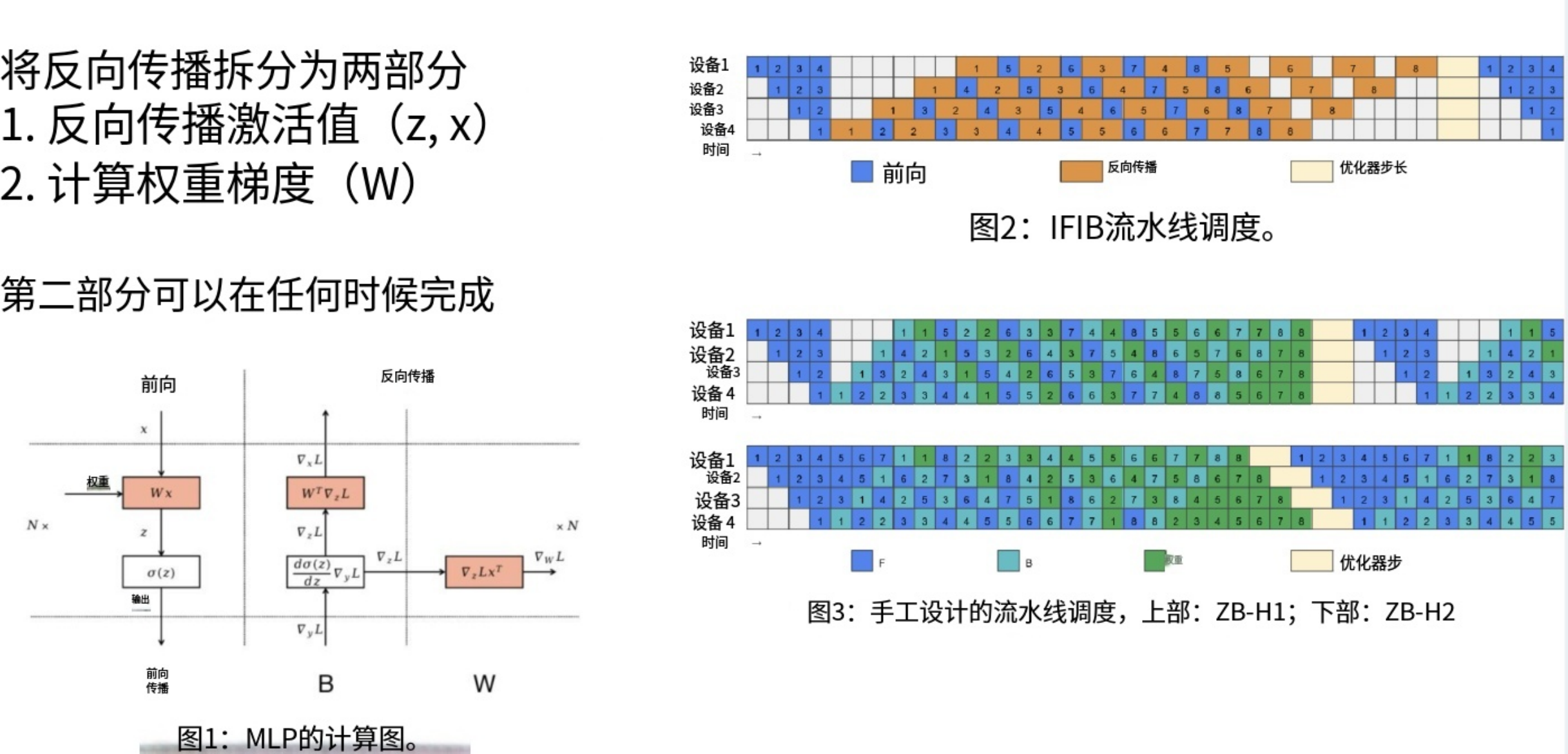
The core idea starts from an optimized 1F-1B pipeline (see Figure 2's 1F1B pipeline scheduling in the figure above), then decomposes it into two parts: this allows inserting W computations at positions where computation bubbles原本 would appear (those white idle regions). Through precise analysis of sequential dependencies, we can ultimately achieve efficient utilization of GPU compute resources.
Let's look at Figure 1: MLP Computation in the bottom left of the above figure. In this diagram, you'll see the forward propagation process (first example, F). This is a simple MLP unit — we first do weight multiplication, then nonlinear transformation, finally output the nonlinear transformation result. This counts as the most basic unit in an MLP. Now look at (second example, B) backward propagation: we get a derivative input with respect to the loss function, then can compute how this derivative changes input x — this is equivalent to computing derivatives with respect to activations here. In the process of computing these derivatives, we can use them to calculate the gradients needed for weight updates.
But the key is this rightmost part (W) — the step of computing gradients for weights — it can actually be done at any time because it has no dependencies. Therefore, this computation can be rescheduled to any position in the computation graph. In specific operations, you can apply standard pipeline parallelism to parts with sequential dependencies. Any computation solely used for updating parameters can be rescheduled to arbitrary positions. Thus, understanding what F, B, W mean, we can see the right-side portion.
Recently, I heard an interesting anecdote: at a certain frontier lab training LLMs, only two people on the team truly understood the infrastructure implementation of pipeline parallelism. After one person left, the entire training infrastructure只剩 one core person supporting it. Such situations确实 exist. Although看起来 simple here, pipeline parallelism is very, very complex at the infrastructure level.
2. Tensor Parallelism
Compared to pipeline parallelism, tensor parallelism is much simpler — many frameworks can implement it, and even teams training ultra-large-scale models primarily rely on this type of model parallelism.
Most of our operations are matrix multiplications. In large models, the vast majority of computation and parameters come from matrix operations. Therefore, if we can parallelize matrix multiplication, the results will be very good. The idea of tensor parallelism is to decompose large matrix multiplications into several sub-matrices that can be computed in parallel.
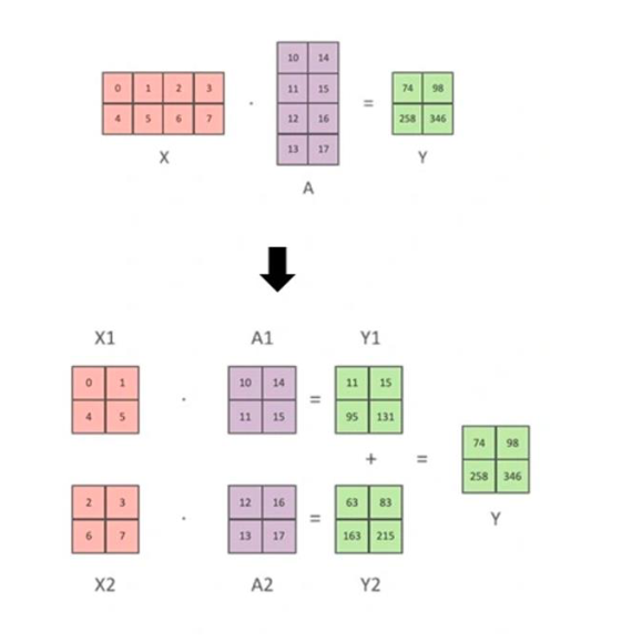
For example, the matrix multiplication
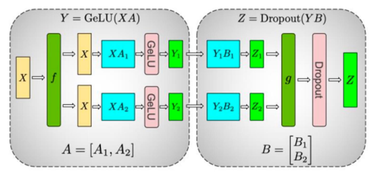
Above is an example in an MLP. Each GPU handles different sub-matrices of the large MLP matrix multiplication, then synchronizes activations via collective communication when needed.
The specific operation: above is an MLP structure — the upper and lower halves represent two different paths for partitioning the matrix. We need to compute
In the left diagram, during forward propagation, input
The f and g here are synchronization points — forward propagation executes one All-Reduce, backward propagation also executes one All-Reduce, just at different positions in the computation graph. From this example, we can see that for any matrix multiplication operation, we can achieve cross-device parallel computation through matrix partitioning.
In tensor parallelism's forward and backward propagation, there are two key synchronization points f and g, which have a dual relationship: Forward propagation: f is identity (directly copy input), g is All-Reduce (sum and aggregate each part's computation results). Backward propagation: g becomes identity (gradient directly passes back), f becomes All-Reduce (sum local gradients from different devices). Understanding this duality is key to correctly implementing tensor parallelism — it determines the specific position of All-Reduce operations in the computation graph.
But it's worth noting that the cost of this method is relatively high, because every layer has a synchronization process — in a single forward-backward pass, we need to transmit twice the residual activation data volume. Therefore, this simple and direct tensor parallelism approach requires high-speed interconnect devices.
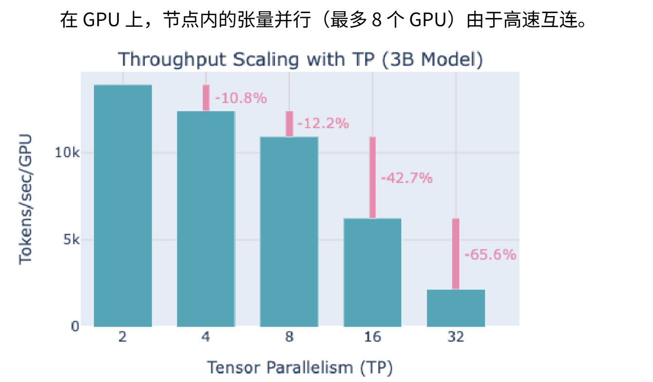
A rule of thumb: tensor parallelism is typically applied within a single node — for example, NVIDIA device boxes with 8 GPUs interconnected via high-speed links enabling fast communication. Using high-bandwidth-demand tensor parallelism schemes among these 8 devices is a reasonable choice, as typically tensor parallelism is deployed across 8 GPUs in a single machine, minimizing performance loss. Hugging Face's parallelization tutorial example (figure above) shows that as tensor parallelism degree increases, throughput progressively drops — at 8 GPUs, there's roughly 10%-12% performance loss, still acceptable; but expanding to 16 devices, a startling 42% performance degradation occurs; at 32 devices, throughput drops another 65%. From visualized data, we can intuitively see that tensor parallelism reaches its optimal balance point at 8 GPUs, determined by hardware interconnect characteristics.
Compared to pipeline parallelism, tensor parallelism doesn't need to handle the pipeline bubble issues mentioned earlier. We don't need to consume larger batch sizes to reduce bubbles, and the complexity of applying tensor parallelism is relatively low. What we truly need to understand is where large matrix multiplications are, whether they can be split and placed on different devices. Forward and backward operations remain unchanged.
The disadvantage is much higher communication overhead. In pipeline parallelism, each micro-batch has point-to-point communication of batch_size × sequence_length × residual_dimension. In tensor parallelism, each layer has 8× communication volume, plus All-Reduce communication — the communication volume needing处理 can be very large. So we have a rule of thumb: tensor parallelism is used in low-latency, high-bandwidth interconnect scenarios. Depending on the machine type owned, in practice, we see 2 to 16-way tensor parallelism.
Also, we can use both parallel strategies simultaneously. We can see that in large-scale operations, tensor parallelism is often used, with pipeline parallelism typically used on top of that. As far as I know, the only example I'm aware of that uses only pipeline parallelism without tensor parallelism is DeepSeek V3. So suppose you have five different machines — perhaps the first 20% of parameters are distributed within one machine's scope using tensor parallelism, then pipeline parallelism moves to the second machine for the next step. Basically, we use tensor parallelism within machines and combine data and pipeline parallelism between machines. Fundamentally, we use pipeline parallelism because your model cannot completely fit in memory. If the entire model can fit in memory, we only need data parallelism plus tensor parallelism, or even just data parallelism.
3. Expert Parallelism
Comparison with Tensor Parallelism
Expert Parallelism is conceptually similar to tensor parallelism — both split MLPs across multiple devices and thus incur communication costs. But they have fundamental differences:
First is partitioning granularity: Tensor parallelism splits a single matrix multiplication across different devices — matrices get smaller and smaller, easily leading to GPU utilization degradation. Expert Parallelism keeps each expert's MLP intact — matrix multiplication dimensions remain unchanged, resulting in higher computational efficiency.
Second is routing differences: MoE layers本来就 route tokens to different experts. Using Expert Parallelism can directly route tokens to experts on target devices — this is far more natural than moving dense large activation matrices in tensor parallelism, and also makes it easier to skip unnecessary computation or overhead.
For this reason, NVIDIA Megatron's official parallelism guide explicitly recommends: between EP and TP, prioritize Expert Parallelism (EP over TP).
Communication Patterns
Expert Parallelism's communication pattern is All-to-All. Each MLP layer needs to distribute tokens to experts on different devices based on routing results, and after computation, results must be sent back. The entire process is extremely latency-sensitive because all devices must wait for tokens to arrive before beginning computation.
This brings enormous engineering complexity. The industry has developed specialized底层 communication libraries for this:
DeepSeek DPP: DeepSeek's expert-parallel routing and distribution library developed for V3, penetrating deep into底层 GPU network primitives, even using undocumented PTX instructions (GPU machine code) to further accelerate communication, squeezing out every last bit of performance. NVIDIA Hybrid EP: Similar底层 library developed by NVIDIA, achieving efficient implementation of expert-parallel distribution at the hardware level.
DP and EP Replica Constraints
When combining Data Parallelism with Expert Parallelism, there's a constraint worth noting. Many older libraries' naive approach: make data-parallel replicas completely overlap with expert-parallel shards. For example, with DP degree 8, place 8 experts分别 on these 8 replicas, with data also sharded and routed across these 8 replicas. This is natural to do, but limits the maximum scale of Expert Parallelism and constrains how DP and TP interact. Modern approaches often require more flexible decoupled designs.
Decoupled Parallelism for Attention and MLP
MoE only replaces MLP layers — attention layers remain dense computation. This creates a contradiction: attention requires relatively high tensor parallelism degree to partition large matrices, but if MoE layers simultaneously use high TP and high EP, matrices get extremely fragmented, causing utilization collapse.
Therefore, in recent years, decoupling strategies have emerged: configuring different tensor parallelism degrees for attention layers vs. MoE layers. For example, attention layers maintain relatively high TP, while MoE layers adopt lower TP or no TP at all (EP-dominant). Although this design is more complex, it can achieve optimal balance among attention, MoE, and data parallelism, and has already been applied in actual frontier models.
4. Sequence Parallelism
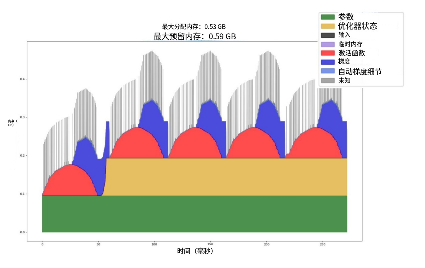
In a sense, memory is a very important part of parallelization, because when training large models, activations actually occupy a large portion of memory usage. In standard forward-backward passes, memory usage is very dynamic. From the figure above, we can see that during training, memory always has static parameters — this portion is unchanging. At iteration zero, since there are no optimizer states yet, that portion of memory usage doesn't exist. But during forward and backward passes, activation memory gradually grows — activations accumulate. When backward pass begins, activation memory decreases because activations are used and released while gradients accumulate. So gradient memory usage rises. The peak actually occurs at a certain stage during backward pass when not all activations have been released while gradients are still accumulating.
The meaning of this diagram: we've considered all other parts — we've considered parameters, optimizer states, and gradients. But we haven't deeply considered activations.
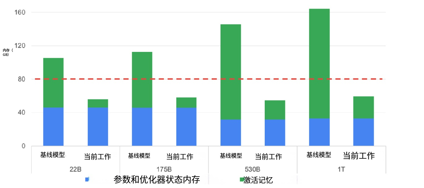
Tensor and pipeline parallelism can linearly reduce most things. But it actually cannot reduce all activation memory usage. The figure above comes from an NVIDIA paper discussing how to reduce activation memory. A very interesting point: reading left to right, models get larger and larger. If aggressive parallelization strategies are adopted, parameter and optimizer state memory can remain constant. But activation memory will continuously grow because certain portions cannot achieve complete parallelization. No matter how many devices, the growth of activation memory on each device cannot be eliminated.
But if more clever methods are adopted (like recomputation, covered in the previous two chapters), activation memory can be maintained at lower levels — and this is crucial for parallelizing certain ultra-large models.
We can compute per-layer activation memory using this convenient formula:
The
Where:
Communication Duality of Sequence Parallelism
Sequence parallelism shards activations of lightweight operations like LayerNorm and Dropout along the sequence dimension. Its communication pattern is similar to FSDP — also a "fetch on demand" approach:
- Forward propagation: Use All-Gather to assemble sharded activations into complete data for computation.
- Backward propagation: Use Reduce-Scatter to distribute gradients back to each device.
Combining tensor parallelism with activation recomputation (e.g., using FlashAttention to eliminate softmax storage), per-layer activation memory can be reduced to the theoretical lower bound:
This is a practical reference value when manually calculating whether a model can fit on GPU.
Assuming full implementation of tensor parallelism (including MLP, KQ computation, and attention operations), per-layer activation memory divided by device count t shows significant effect, but there's still an
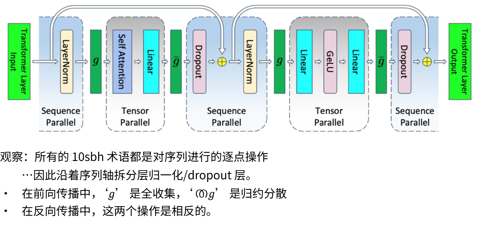
Finally, we need to handle the previously unparallelized simple pointwise operations. Taking layer normalization as an example — normalization at different positions in the sequence doesn't interfere with each other. Suppose sequence length is 1024 — we can partition it and have different devices respectively handle layer normalization or Dropout operations. These pointwise operations can now be completely partitioned along the sequence dimension, but synchronization mechanisms are needed to aggregate parallel computation results — forward propagation uses All-Gather, gradient backward propagation uses Reduce-Scatter, forming a dual relationship. The specific flow: during layer normalization, scatter data then reaggregate to execute standard computation; during Dropout, scatter again to parallel components. During backward propagation, execute in reverse order.
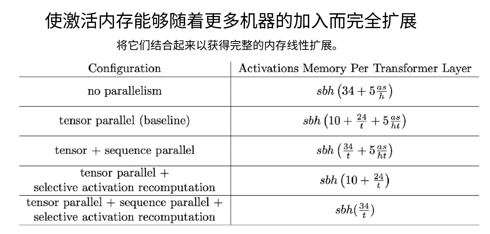
This approach called Sequence Parallelism is essentially the final optimization for previously unparallelized components. Now integrating all modules — starting from complete no-parallelism, first use tensor parallelism to divide all non-pointwise operation memory by t, then apply the sequence parallelism concept to divide remaining component memory again by t, ultimately achieving comprehensive optimization. Then we can do things like activation recomputation — this is FlashAttention's trick — to eliminate the second term. The minimum memory you can easily achieve will be the formula at the bottom:
8.2.3 Other Parallel Strategies
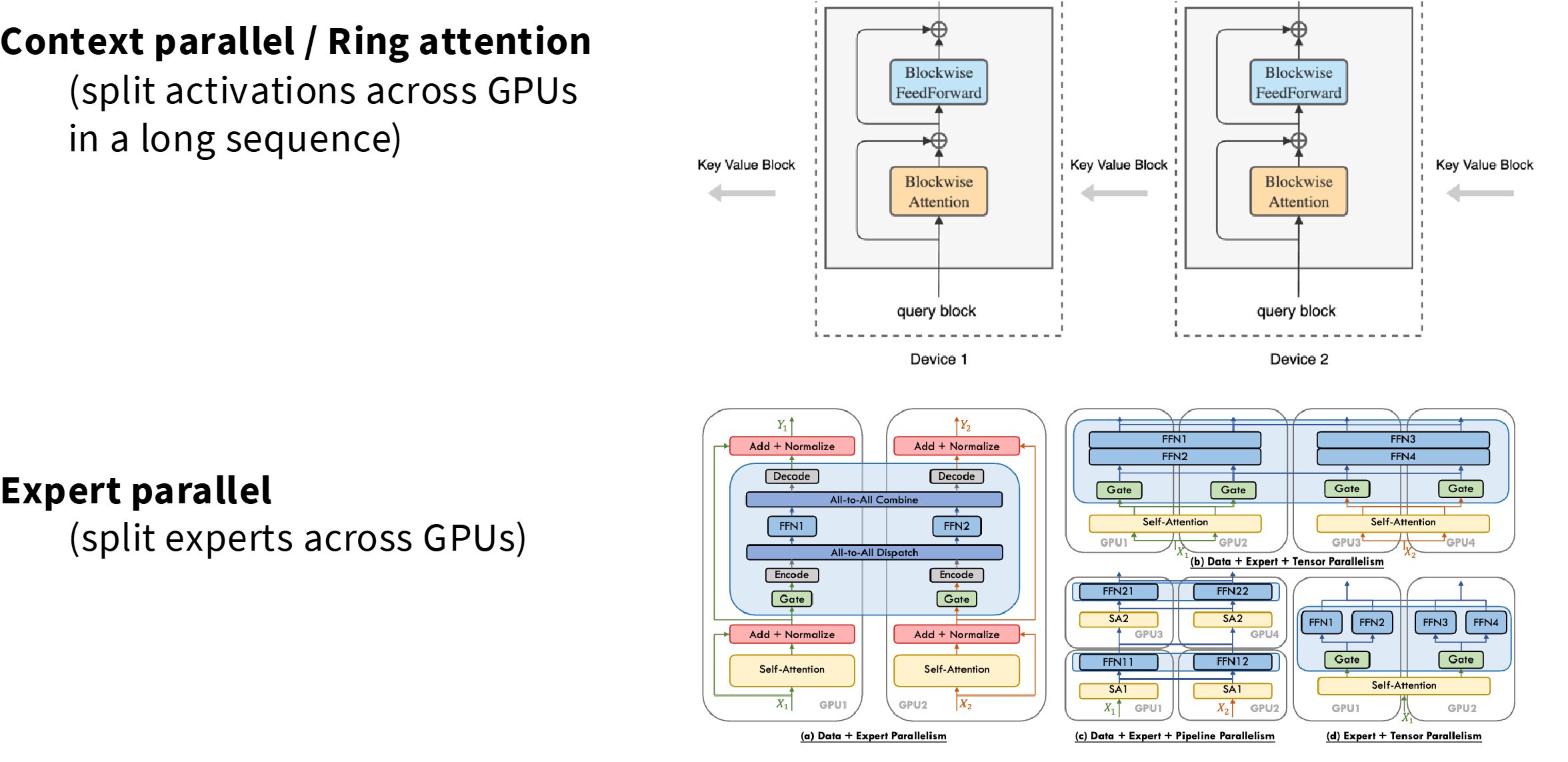
Context Parallelism or Ring Attention — this is essentially a method for splitting computation and activation costs for computing very large attention, basically having keys and values pass between different machines. So each machine is responsible for different queries Q, and keys and values will be transferred between machines in a ring fashion to compute KQV inner products.
Context parallelism is specifically designed to address the challenge of ultra-long sequence training. It splits queries Q across different devices, while keys K and values V are passed sequentially between devices in a ring fashion — each device only computes a portion of attention scores, thereby avoiding instantiating the complete attention matrix on any device. This is in line with FlashAttention's tiled computation philosophy and is commonly used for long-context extension training. For example, Llama 3 during the long-context fine-tuning phase increased context parallelism degree from 1 to 16 while reducing data parallelism degree to free up memory.
We've done tiling in FlashAttention. So we know attention can be computed in this online tile-by-tile manner.
8.2.4 Summary
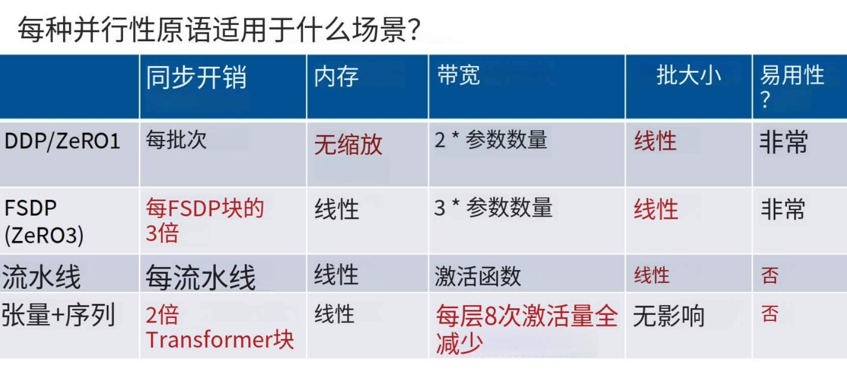
So briefly reviewing everything we've discussed: We have DDP in ZeRO-1, which is somewhat like naive data parallelism. Each batch has some overhead, no memory scaling, reasonable bandwidth characteristics, but requires consuming batch size to achieve this — we need large batch sizes for large data parallelism.
There's also FSDP, which is a better version of ZeRO-1, because it achieves memory scaling, but pays overhead between different layers. So now there's higher communication cost and possibly synchronization barriers causing low utilization.
FSDP, although total communication reaches 3× parameter count (one more All-Gather than DDP), can maintain near-single-card efficiency. The key is communication-computation overlap: the CPU scheduler pre-initiates All-Gather requests to prefetch the next layer's parameters — while the current layer computes, the next layer's data is already ready in the background. This multi-stream pipeline design hides the vast majority of communication latency beneath computation time, with actual performance loss typically only 10%~20%.
Pipeline parallelism's advantage: we no longer depend on batch size — we can achieve linear memory scaling. But we have another problem: this also consumes batch size, and it's very troublesome to set up and use. So if possible, many people prefer to avoid pipeline parallelism.
Tensor parallelism is very expensive in terms of bandwidth and the amount of synchronization needed. But it has one very nice property: no impact on batch size. So this is a parallel strategy that can be used because it has no cost in terms of global batch size. So we must balance limited resources — memory, bandwidth, and compute. Batch size is a non-traditional and finite resource.
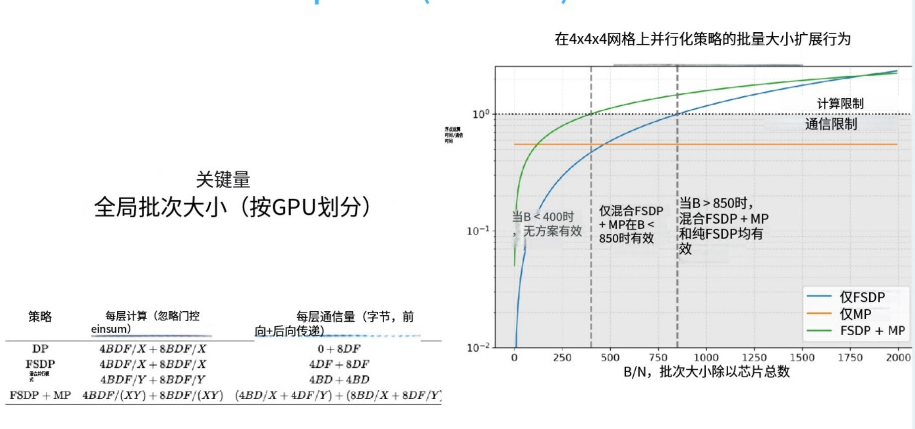
Observing the chart above, we can see the key quantity is batch size. Based on the ratio of batch size to GPU count, different parallel strategies achieve optimal effectiveness. They compute communication volume and computation volume for each model type through specific formulas — this chart is generated from simplified formulas. We can clearly see: when batch size is too small and GPU count too high, system efficiency is necessarily low because it's始终 limited by communication bottlenecks — i.e., the lower portion of the chart, where most time is spent on communication. As batch size gradually increases, when combining FSDP (i.e., ZeRO Stage 3) with tensor parallelism (MP), we ultimately achieve a compute-bound state. At this point, compute units no longer waste floating-point capability waiting for communication. When batch size is sufficiently large, pure data parallelism alone suffices, because pure FSDP makes compute time significantly higher than communication time. This diagram vividly illustrates the value of hybrid parallel strategies: when hybridization is needed, and why batch size belongs in the resource category.
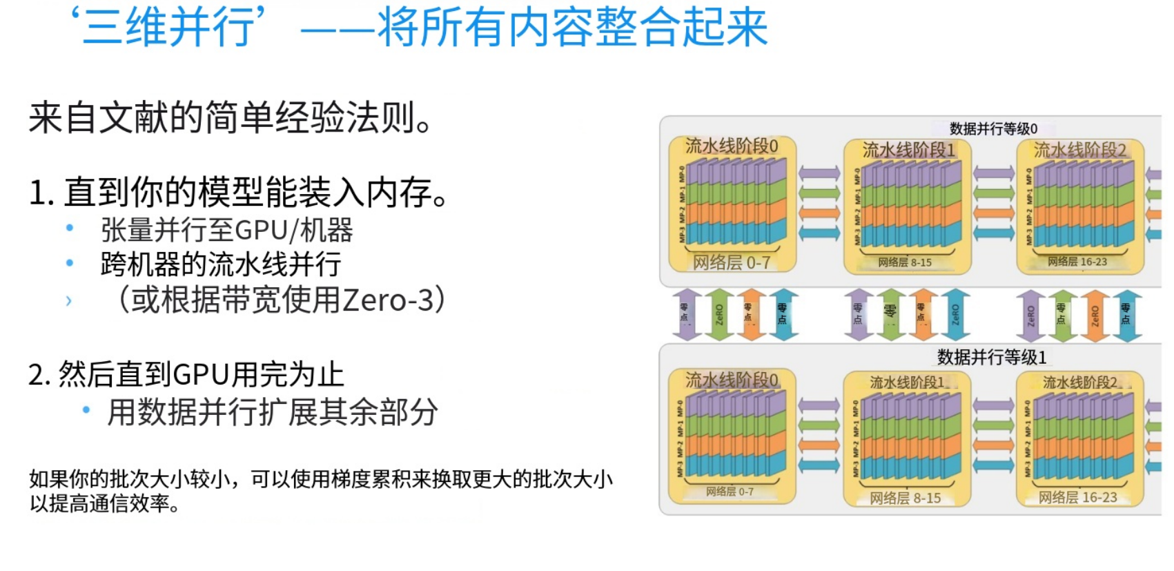
When integrating all parallel dimensions, we form what's called a 3D or 4D parallel scheme (5D parallel concepts have even emerged recently). Although the specific meaning of the fifth dimension awaits verification, existing dimension combinations already form concise and practical rules of thumb. The primary principle: ensure the model and activations can be accommodated by memory — this is the prerequisite for training. When single-machine memory is insufficient, first adopt tensor parallelism — within the range of single-machine GPU count, this is the most efficient scheme. Then based on pipeline parallelism applicability and bandwidth constraints, adopt ZeRO-3 or pipeline parallelism across machines until the model is fully loaded into memory.
Before GPU resources are exhausted, all remaining scaling is achieved through data parallelism, because this方案 both adapts to low-bandwidth environments and is simple to implement. If batch size is small, gradient accumulation techniques can achieve effectively large batch processing, thereby improving communication efficiency (reducing inter-machine synchronization frequency). This methodology ensures model training always maintains reasonable efficiency.
To concretely illustrate, let's show a few typical cases

Visual论证 from a 2021 paper (with extensive ablation experiments), plus practical data from some models last year. This model training table spanning 1.7B to 1T parameters shows that all approaches achieved 40%-52% of theoretical peak floating-point utilization.
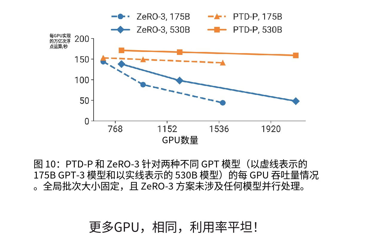
We can clearly see: tensor parallelism starts at 1, gradually increases to 8, then caps; pipeline parallelism initially at 1, only gradually increases as the model膨胀; data parallelism scale starts at maximum and progressively decreases — because increasing pipeline parallelism essentially consumes batch capacity. Therefore, if GPUs are某种程度上 used for pipeline parallelism, we cannot effectively achieve such large batch sizes. So carefully designed 3D parallel strategies bring linear growth in aggregate floating-point operations.
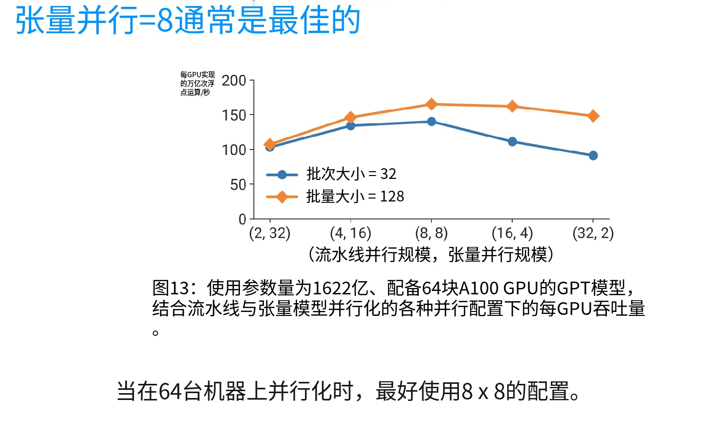
Through精细的 3D parallel configuration, each GPU can maintain very stable actual compute performance — this means adding GPUs achieves linear scaling of total throughput, which is very ideal. Tensor parallelism set to 8 is typically the optimal solution. Shown here is the correspondence between pipeline parallelism scale and tensor parallelism scale. We can see when tensor parallelism is set to 8,配合 batch size of 128 gives the best results. Even with smaller batch sizes, keeping the tensor parallelism dimension at 8 remains the optimal choice.
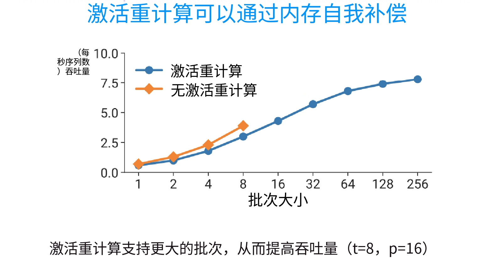
Activation recomputation technology can support larger batch sizes. Notably, larger batches in turn help hide pipeline parallelism overhead. Therefore, although activation recomputation increases computation, its benefits are足以 offset the costs. We've already witnessed this phenomenon in FlashAttention. Next, let's discuss practical approaches from recent LLMs.
Multiple papers reveal commonly used parallelization strategies in industry: OLMo and Dolma papers describe using Fully Sharded Data Parallelism (FSDP) for their 7B parameter model; DeepSeek's initial paper uses ZeRO Stage 1配合 tensor, sequence, and pipeline parallelism — exactly the basic scheme I introduced earlier. The V3 version is slightly different: adopting 16-way pipeline parallelism + 64-way expert parallelism (essentially a tensor parallelism variant), with data parallelism using ZeRO Stage 1. Another domestic model Yi again uses ZeRO Stage 1 with tensor/pipeline parallelism; Yi-lightning, being a MoE model, replaces tensor parallelism with expert parallelism.
Small-batch initial phase training is for ensuring stability and can also be ignored. By analyzing their parallel strategy design logic, you'll find it完全印证了 our discussion: sorted by bandwidth requirements, prioritize TP -> CP -> Pipeline Parallelism -> DP, because data parallelism tolerates higher network latency and supports asynchronous fetching of sharded model parameters. They正是运用 this strategy suite to train certain top-tier models.
An interesting anecdote about Llama 3: during ultra-large-scale training, GPU failures are frequent. 148 training interruptions were caused by faulty GPUs, accounting for 30% of total interruptions. There were also 32 other types of unexpected situations like emergency machine maintenance. When training such enormous models, besides algorithm design, we also need to build fault-tolerant architectures to handle these challenges. But what's truly worrisome isn't显性 model failures — it's silent data corruption: GPUs may output garbage data without any warning, directly destroying the entire training run.
In ultra-large-scale training, GPU hardware failures are the norm. According to Meta's report, during Llama 3 405B training, 148 GPU failures occurred, accounting for 30% of total interruptions. A more隐蔽 threat is Silent Data Corruption: GPUs may output incorrect results without any error reporting, directly破坏 the training process. Therefore, training systems must not only be fast at parallelism but must also build in redundant fault tolerance and automatic recovery mechanisms — a major challenge at the distributed systems level.
Gemma 2 is also a typical TPU case — they adopt近似 FSDP's ZeRO Stage 3, combining model parallelism with data parallelism. TPU architecture allows greater degrees of model parallelism.
Overall, to achieve ultra-large-scale scaling, multi-GPU multi-node parallel schemes are essential. There's no single万能 solution — we need to融合 three parallel approaches, leveraging their respective strengths. In practice, simple and interpretable rules of thumb exist to guide parallel strategy implementation.
Parallel Configurations in Actual Training Cases
| Model | Parallel Strategy Combination | Details |
|---|---|---|
| DeepSeek V1 | ZeRO-1 + TP + SP + PP | Standard dense model strategy |
| DeepSeek V3 | ZeRO-1 + 16 PP + 64 EP | Large-scale EP replacing TP, MoE model |
| Yi (dense) | ZeRO-1 + TP + PP | Classic triple combo |
| Yi-lightning (MoE) | EP replacing TP | Strategy adjustment after MoE conversion |
| Llama 3 405B | Pretrain: TP=8, CP=1, PP=16, DP=128 | Long-context phase: CP→16, DP reduced |
| Mixtral 8×22B | EP=8, PP=4, TP=4 | TP for decoupled attention layers |
| Gemma 2 (TPU) | FSDP + TP + SP, no PP | Leveraging TPU large mesh high bandwidth, no pipeline needed |
| Qwen 3 | EP=32, PP=8, TP=2 | Following DeepSeek's high EP route |
| OLMo 7B | Pure FSDP | Small model only needs FSDP |
8.3 Multi-GPU Parallel Optimization and Distributed Training System Practice
8.3.1 Fundamental Building Blocks
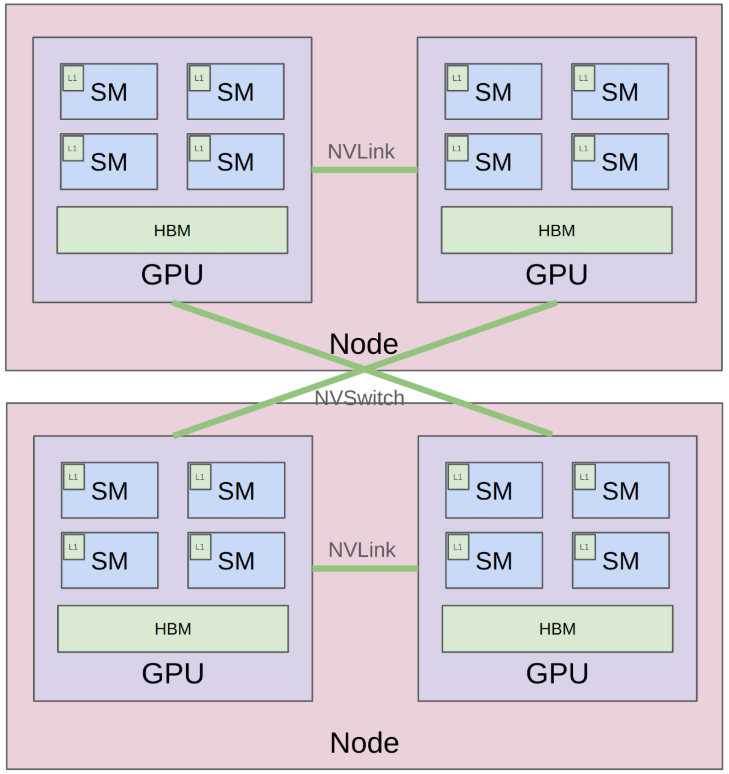
We'll explore parallelization across multiple GPUs. Everyone should have an architecture diagram like the one above in mind. It has multiple nodes, which are essentially computers, each equipped with若干 GPUs, typically 8. Each GPU internally contains multiple Streaming Multiprocessors (SMs), where actual computation work happens. The green portions in the diagram represent memory and communication components. Each SM internally has minimal L1 cache, GPUs are equipped with larger-capacity High Bandwidth Memory (HBM), and there are interconnect links connecting different GPUs (those green lines).
The core idea: computation must occur on the Arithmetic Logic Units (ALUs) inside SMs. The computation process requires reading inputs and writing outputs, and typically input/output data may be located relatively far away — ideally in L1 cache, suboptimal in HBM. And in the multi-GPU/multi-node training we're discussing now, needed data may be located on other GPUs. Therefore, the key is how to design computation structures to avoid data transfer bottlenecks.
The core goal: maintain high arithmetic intensity, keep GPUs fully loaded. Since data transfer is typically much slower, it's the primary bottleneck. We previously learned GPU-internal optimization techniques (like operator fusion and memory tiling) — their core idea is avoiding direct HBM reads/writes, instead loading data into L1 cache (or equivalently fast shared memory), completing computation in local registers后, then carefully writing back to HBM. This time, we'll focus on cross-GPU/node communication, involving model parameter replication and sharding, state optimization, etc. — these implementation approaches will directly determine communication costs.
Fastest and smallest is single-GPU L1 cache; next is single-GPU HBM; then intra-node GPU-to-GPU NVLink; finally NVSwitch (of course, this整套 belongs to the NVIDIA ecosystem). This time, we'll focus on concretizing theoretical concepts through code implementation. We've excellently outlined various parallelization approaches above. We'll attempt to anchor these concepts through code for deeper understanding of implementation principles.
This first part explores fundamental building blocks — collective communication operations, including NCCL and PyTorch implementation approaches, with benchmarking. The second part practically studies data parallelism, tensor parallelism, and pipeline parallelism in distributed training.
8.3.2 Collective Communication Primitives
Now starting with collective communication operations. These primitives are widely used in distributed programming — "collective" means involving multiple nodes. These concepts are actually very old, traceable to at least 1980s parallel programming literature. Compared to managing point-to-point communication oneself, they provide more elegant abstraction and are time-tested reliable primitives.
First, clarify terminology:
World size refers to total device count, rank simply indicates device number (distinguish from the rank concept in linear algebra). With four devices, ranks are 0, 1, 2, 3 respectively.
Collective communication operations include:
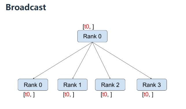
Broadcast means distributing tensor t0 from a certain rank to all ranks;
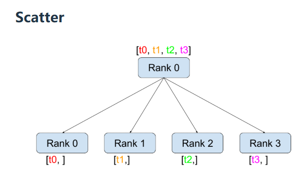
Scatter is similar but sends four different values to different ranks respectively. So each rank receives different values, not the same value.
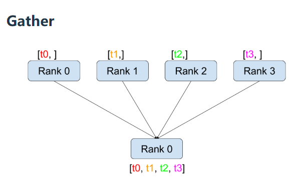
Gather is the inverse of scatter — each rank has different values, then汇集 them onto one rank.
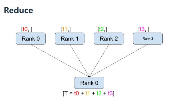
Reduce is similar to gather, except instead of concatenation, values are summed.
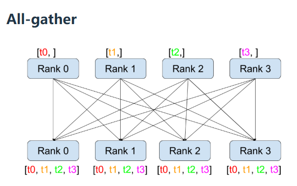
All-Gather is the same as gather, except it's executed for all target ranks.
Gather only targets rank 0, rank 1, rank 2, or any single rank.
All-Gather is executed for all ranks.
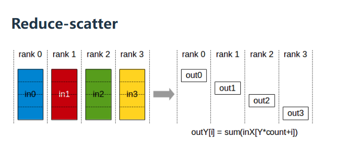
Reduce-Scatter — reusing the earlier diagram, similar to reduce — takes a set of different values, sums them or performs other associative operations, and places the result on one rank.
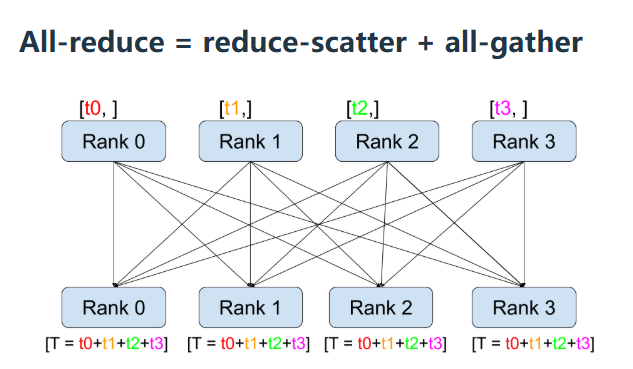
All-Reduce is equivalent to reduce plus All-Gather.
Reduce only means you perform some associative and commutative operation like sum, min, max, or average. Broadcast/scatter is the inverse of gather. And "all" simply means the target is all devices. Hopefully, this is review of the content.
8.4 Hardware Architecture and Communication Hierarchy
8.4.1 GPU Hardware Architecture
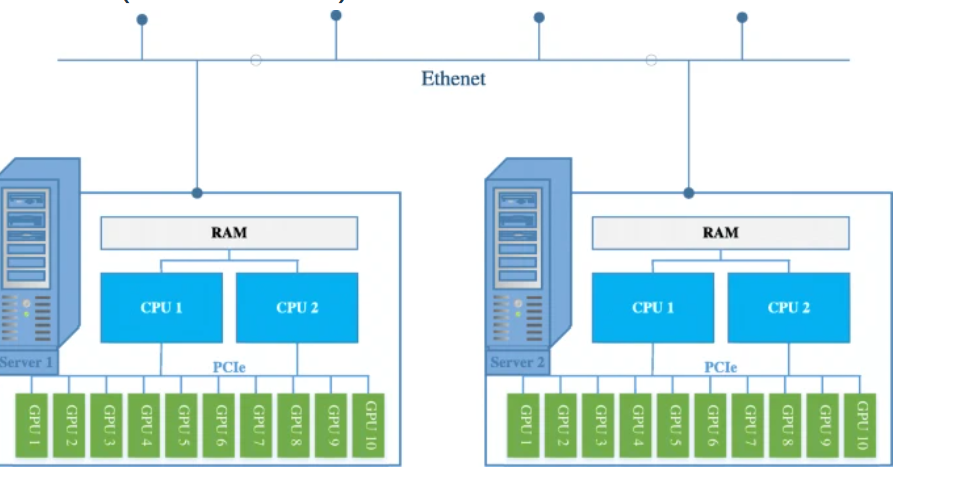
Starting with hardware. Above is a typical GPU hardware architecture: in a home environment, a computer has a CPU, and on the node, GPUs communicate via PCI-E bus. If communication between different nodes is needed, it goes through Ethernet. GPUs on the same node communicate via PCI(e) bus (v7.0, 16 lanes => 242 GB/s), GPUs on different nodes communicate via Ethernet (~200 MB/s). If we buy GPUs for gaming or other purposes, this is what our setup looks like.
PCI-E data still must pass through the CPU. PCI-E was developed for connecting other devices like sound cards, SSDs, or hard drives. So it wasn't specifically designed for GPUs — it's a general-purpose device communication bus.
But this isn't ideal because there's a lot of overhead. For instance, when data needs to transfer from GPU to GPU, it must pass through the kernel, be copied to buffers, then transmitted via Ethernet — this introduces lots of overhead. Therefore, in modern scientific computing and deep learning, if we connect a bunch of GPUs together to jointly execute tasks, we directly connect GPUs.
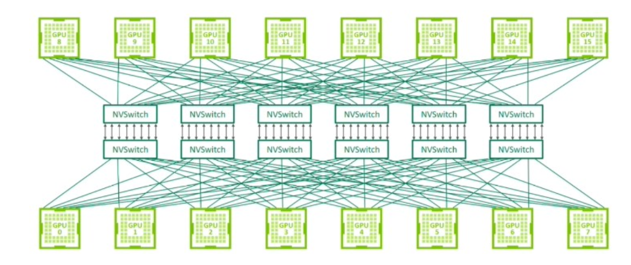
In the NVIDIA ecosystem, we have NVLink directly connecting GPUs, thereby bypassing the CPU — no need to go through the host kernel. Even cross-node, we can directly connect GPUs via NVSwitch. Thus bypassing Ethernet, because Ethernet was developed long ago and显然 wasn't designed for these applications. So NVSwitch and NVLink skip all of this, directly optimizing for the workload types we're interested in.
If you look at the H100, each GPU has 18 fourth-generation NVLinks. This provides a total of 900 GB bandwidth. It's certainly much faster than PCI-E and Ethernet. But considering the cost of reading from SM to High Bandwidth Memory, HBM memory bandwidth is 3.9 TB/s — that's still about 4× faster. With the new Blackwells launching, it will increase by another 2-3×.
8.4.2 NCCL
NVLink still needs to communicate with the CPU. Each GPU pair has NV18 connections, plus these network card things — network cards essentially provide PCI-E connections and CPU components.
NVIDIA spent大量 time developing very excellent software on top of their excellent hardware. They developed a collective communication library called NCCL, which essentially converts the collective operations we discussed earlier (e.g., All-Reduce) into low-level data packets that need to be transferred between GPUs. This library actually undertakes大量 work because it lets programmers operate at the level of "I need this tensor to appear on all machines," and then it automatically实现.
Brief explanation of its operational principle: When you configure and launch NCCL, it activates a set of devices. The system probes hardware topology through communication, optimizing transfer paths between GPUs. When you actually call these collective communication operations, it launches CUDA kernels to send and receive data.
It's provided as a library. But NCCL's usage level is still somewhat low, since most of our work is in Python. Therefore, PyTorch provides the torch.distributed library, essentially offering简洁 interfaces for these collective operations. You can easily write All-Gather and other operations in PyTorch programs, and tensors automatically appear across all processes of different ranks. It also has the nice feature of supporting multiple hardware backends. Especially remember NCCL is for GPU, but collective operations aren't limited to GPU — they apply to any device collection. You can also run on CPU using the backend called gloo. For instance, when debugging assignments on a laptop, even without GPU, it can run normally through gloo. This is another advantage of having high-level primitives — they have better portability than solutions limited to GPU-specific functionality. Of course, actual performance depends on hardware, but at least it ensures code logically runs correctly. The distributed library also supports other high-level features like FSDP (covered above).
Let's look at some practical examples of torch.distributed collective operations
spawn(collective_operations_main, world_size=4)The utility function above takes a function and launches four processes to execute it through a Python multiprocessing wrapper. When running this function, you should understand that there are world_size processes executing the same function, with rank indices from 0 to world_size minus 1.
def setup(rank: int, world_size: int):
    # Specify where the master server is located (rank 0), used for coordination (actual data goes through NCCL)
    os.environ["MASTER_ADDR"] = "localhost"
    os.environ["MASTER_PORT"] = "15623"
    if torch.cuda.is_available():
        dist.init_process_group("nccl", rank=rank, world_size=world_size)
    else:
        dist.init_process_group("gloo", rank=rank, world_size=world_size)

def cleanup():
    torch.distributed.destroy_process_group()

def collective_operations_main(rank: int, world_size: int):
    """This function runs asynchronously for each process (rank = 0, ..., world_size - 1)."""
    setup(rank, world_size)

    # All-reduce
    dist.barrier()  # Waits for all processes to get to this point
    tensor = torch.tensor([0., 1, 2, 3], device=get_device(rank)) + rank  # Both input and output
    print(f"Rank {rank} [before all-reduce]: {tensor}", flush=True)
    dist.all_reduce(tensor=tensor, op=dist.ReduceOp.SUM, async_op=False)  # Modifies tensor in place
    print(f"Rank {rank} [after all-reduce]: {tensor}", flush=True)

    # Reduce-scatter
    dist.barrier()
    input = torch.arange(world_size, dtype=torch.float32, device=get_device(rank)) + rank  # Input
    output = torch.empty(1, device=get_device(rank))  # Allocate output
    print(f"Rank {rank} [before reduce-scatter]: input = {input}, output = {output}", flush=True)
    dist.reduce_scatter_tensor(output=output, input=input, op=dist.ReduceOp.SUM, async_op=False)
    print(f"Rank {rank} [after reduce-scatter]: input = {input}, output = {output}", flush=True)

    # All-gather
    dist.barrier()
    input = output  # Input is the output of reduce-scatter
    output = torch.empty(world_size, device=get_device(rank))  # Allocate output
    print(f"Rank {rank} [before all-gather]: input = {input}, output = {output}", flush=True)
    dist.all_gather_into_tensor(output_tensor=output, input_tensor=input, async_op=False)
    print(f"Rank {rank} [after all-gather]: input = {input}, output = {output}", flush=True)

    # Indeed, all-reduce = reduce-scatter + all-gather!
    cleanup()
All-Reduce
    # All-reduce
    dist.barrier()
    tensor = torch.tensor([0., 1, 2, 3], device=get_device(rank)) + rank
    print(f"Rank {rank} [before all-reduce]: {tensor}", flush=True)
    dist.all_reduce(tensor=tensor, op=dist.ReduceOp.SUM, async_op=False)
    print(f"Rank {rank} [after all-reduce]: {tensor}", flush=True)
In the typical flow, processes first need to initialize themselves. Multiple processes need to discover each other — they connect to the same host to confirm each other's existence (using setup). Note this isn't the data transfer channel (data goes through NCCL) — this is just the coordination mechanism. Since we have GPUs, we use the NCCL backend; otherwise, we'd use gloo. After initialization completes, we begin actual operations.
There's a useful barrier function (dist.barrier()), which waits for all processes in the process group to reach this synchronization point. All operations run asynchronously, so synchronization points need to be established — barrier serves this purpose. Here, it's used to group print statements for display; we'll see other use cases later.
tensor = torch.tensor([0., 1, 2, 3], device=get_device(rank)) + rank creates a tensor for each process group — content is 0123 plus the current rank value. Before executing the all-reduce operation, print each rank's tensor state.
Now showing results:
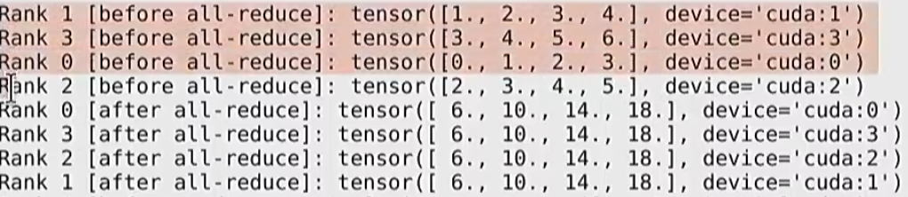
Rank 0 shows 0123, rank 1 shows 1234, and so on. Note that due to asynchronous execution, the print order is out of order. Each rank has different tensors, then executes the all-reduce operation: dist.all_reduce(tensor=tensor, op=dist.ReduceOp.SUM, async_op=False) — passes in the tensor and specifies sum operation. In this case, not using asynchronous operations, but asynchronous mode can be adopted, which is useful for overlapping communication and computation. After the all-reduce operation, as printed out, for the first component (first four rows), they sum to 6. The last four rows show sums of 10, 14, and 18. So after all-reduce, this tensor is basically overwritten by the corresponding sums. Very, very简洁 and convenient to use.
Reduce-Scatter
    # Reduce-scatter
    dist.barrier()
    input = torch.arange(world_size, dtype=torch.float32, device=get_device(rank)) + rank
    output = torch.empty(1, device=get_device(rank))
    print(f"Rank {rank} [before reduce-scatter]: input = {input}, output = {output}", flush=True)
    dist.reduce_scatter_tensor(output=output, input=input, op=dist.ReduceOp.SUM, async_op=False)
    print(f"Rank {rank} [after reduce-scatter]: input = {input}, output = {output}", flush=True)
Now demonstrating reduce_scatter. For reduce_scatter, create an input with dimension world_size — here world_size is 4. Then allocate an output, because reduce_scatter doesn't operate in place — the output will be a scalar.

Before reduce_scatter, the data is the first four rows of the above figure — the input is the same as before, and the output happens to be 0, but since it's uninitialized, it could be any value. After executing reduce_scatter, when passing input and output and performing summation, the result is the last four rows. For the first column, after summation, the result is placed on rank 0; the second column after summation is placed on rank 1, and so on. As you've noticed, it performs exactly the same operation as all_reduce, except the output is scattered across all different ranks.
All-Gather
    # All-gather
    dist.barrier()
    input = output  # Input is the output of reduce-scatter
    output = torch.empty(world_size, device=get_device(rank))
    print(f"Rank {rank} [before all-gather]: input = {input}, output = {output}", flush=True)
    dist.all_gather_into_tensor(output_tensor=output, input_tensor=input, async_op=False)
    print(f"Rank {rank} [after all-gather]: input = {input}, output = {output}", flush=True)
Now let's demonstrate all_gather. We'll directly use reduce_scatter's output as input, then allocate an empty array for output.

Before all_gather (first four rows), output is an arbitrary value. After executing all_gather (last four rows), all these tensors appear on all devices. This is just an example. Hopefully, you're now fully convinced that reduce_scatter plus all_gather equals all_reduce, because it computes exactly the same results as all_reduce.
Finally, when the process finishes running, simply perform cleanup.
8.5 Benchmarking
So far, we've discussed these collective communication operations and their implementation in PyTorch, involving NCCL and PyTorch. Now let's do some benchmarking.
def all_reduce(rank: int, world_size: int, num_elements: int):
    setup(rank, world_size)
    # Create tensor
    tensor = torch.randn(num_elements, device=get_device(rank))
    # Warmup
    dist.all_reduce(tensor=tensor, op=dist.ReduceOp.SUM, async_op=False)
    if torch.cuda.is_available():
        torch.cuda.synchronize()  # Wait for CUDA kernel to complete
        dist.barrier()            # Wait for program to reach here
    # Perform all-reduce
    start_time = time.time()
    dist.all_reduce(tensor=tensor, op=dist.ReduceOp.SUM, async_op=False)
    if torch.cuda.is_available():
        torch.cuda.synchronize()  # Wait for CUDA kernel to complete
        dist.barrier()            # Wait for program to reach here
    end_time = time.time()
    duration = end_time - start_time
    print(f"[all_reduce] Rank {rank}: all_reduce(world_size={world_size}, num_elements={num_elements}) took {render_duration(duration)}", flush=True)

    # Measure bandwidth
    dist.barrier()
    size_bytes = tensor.element_size() * tensor.numel()
    sent_bytes = size_bytes * 2 * (world_size - 1)  # 2x because send input and receive output
    total_duration = world_size * duration
    bandwidth = sent_bytes / total_duration
    print(f"[all_reduce] Rank {rank}: all_reduce measured bandwidth = {round(bandwidth / 1024**3)} GB/s", flush=True)
    cleanup()
Taking all_reduce as an example: create a tensor with 100 million elements, world_size is 4. First, allocate the tensor. Note: when benchmarking, you must carefully clean up the environment. Here, I warm up first — run the operation once, then synchronize and execute dist.barrier(), ensuring all kernels are loaded and needed computation is complete.
Then start timing, execute all_reduce, synchronize again, then stop timing. Below, we can查看 the time consumption.

Microseconds should be used here — milliseconds aren't intuitive. But it executes very fast.
    # Measure bandwidth
    dist.barrier()
    size_bytes = tensor.element_size() * tensor.numel()
    sent_bytes = size_bytes * 2 * (world_size - 1)  # 2x because send input and receive output
    total_duration = world_size * duration
    bandwidth = sent_bytes / total_duration
    print(f"[all_reduce] Rank {rank}: all_reduce measured bandwidth = {round(bandwidth / 1024**3)} GB/s", flush=True)
    cleanup()
Now measure bandwidth — i.e., total gigabytes actually transferred per second. The calculation method needs to consider the actual amount of data transferred: size_bytes = tensor.element_size() * tensor.numel() — this tensor's element count multiplied by each element's size (here float32, 4 bytes), giving total bytes.
Here's a detail: what's the actual number of bytes sent/received? Each rank's tensor size is size_bytes, needing to send to other world_size-1 ranks. But there's a factor of 2 because during all_reduce (sending all different elements to the same location for summation, then results need to return to all nodes), each compute node needs to first send input, then receive output — this is why there's a factor of 2. Therefore, total duration is world_size multiplied by actual elapsed time.

Bandwidth is bytes divided by duration. Our result is approximately 277 GB/s. Earlier, we mentioned H100 has bandwidth of approximately 900 GB/s. Actual performance varies with tensor size, device count, and various other factors — multiple variables exist. So actual performance may differ — it's best to confirm actual GB/s values through benchmarking.
def reduce_scatter(rank: int, world_size: int, num_elements: int):
    setup(rank, world_size)
    # Create tensor
    input = torch.randn(world_size, num_elements, device=get_device(rank))  # Each rank has a matrix
    output = torch.empty(num_elements, device=get_device(rank))
    # Warmup
    dist.reduce_scatter_tensor(output=output, input=input, op=dist.ReduceOp.SUM, async_op=False)
    if torch.cuda.is_available():
        torch.cuda.synchronize()
        dist.barrier()
    # Perform reduce-scatter
    start_time = time.time()
    dist.reduce_scatter_tensor(output=output, input=input, op=dist.ReduceOp.SUM, async_op=False)
    if torch.cuda.is_available():
        torch.cuda.synchronize()
        dist.barrier()
    end_time = time.time()
    duration = end_time - start_time
    print(f"[reduce_scatter] Rank {rank}: reduce_scatter(world_size={world_size}, num_elements={num_elements}) took {render_duration(duration)}", flush=True)

    # Measure bandwidth
    dist.barrier()
    data_bytes = output.element_size() * output.numel()
    sent_bytes = data_bytes * (world_size - 1)
    total_duration = world_size * duration
    bandwidth = sent_bytes / total_duration
    print(f"[reduce_scatter] Rank {rank}: reduce_scatter measured bandwidth = {round(bandwidth / 1024**3)} GB/s", flush=True)
    cleanup()
The reduce_scatter operation will be very similar — let's quickly go through it: we create world_size times the element count as input, with each compute node owning this matrix. First warm up, then start timing, execute reduce_scatter, stop timing, and compute duration.
Let's look at the bandwidth calculation. Here, the sent bytes also have a factor of 2, because reduce_scatter essentially sends input to specified locations. If only considering the reduce operation, all elements would聚集 at one place; scatter means different portions of the tensor are distributed to different locations, but it's still essentially类似 a reduce operation.

Computing the same way, the result here is approximately 70. Not sure why exactly 70 rather than some other value — possibly because all_reduce typically generates more communication traffic, and all_reduce may have more optimization. NVIDIA hardware has acceleration technology that can perform partial computation in the actual network, saving half the time, but不确定 whether this fully explains the difference here.
NCCL internal implementation is complex, making it difficult to precisely deduce performance — hence the need for benchmarking. To be clear, we assume input data already exists on the device, so that time isn't counted — only the operations needed to execute reduce_scatter are computed.
By comparison, we can see that reduce_scatter and all_gather each don't contain the 2× factor individually — only when combined do they produce the 2× factor, which also confirms that all_reduce requires 2× communication volume. Detailed reference materials on benchmarking and collective operations are available for consultation.
8.6 Distributed Training
We'll demonstrate each strategy through a simple implementation of a deep MLP. It's worth noting that in Transformers, the MLP is typically the computational bottleneck rather than the attention mechanism. Therefore, despite the simple architecture, it well represents the actual workload types.
First, start with data parallelism. To clarify: data parallelism, tensor parallelism, and pipeline parallelism can be understood as different ways of partitioning the model or data — we'll visualize this shortly.
8.6.1 Data Parallelism in Practice
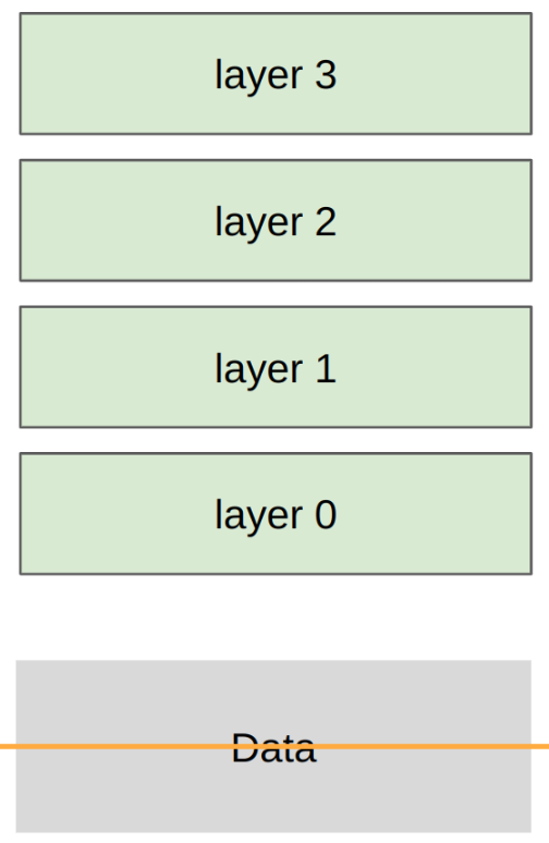
In data parallelism, assume the model contains four layers, each MLP layer being a matrix multiplication operation. Data is also in matrix form (batch dimension × hidden dimension). Data parallelism partitions data along the batch dimension into smaller shards, with each compute node receiving different data slices.
Let's illustrate through an example. Suppose my batch size is 128, hidden dimension is 1024, then randomly generate some data. Data dimensions are batch size × feature dimension. Next, I'll run this data parallelism algorithm (DDP).
# Generate sample data
def generate_sample_data():
    batch_size = 128
    num_dim = 1024
    data = torch.randn(batch_size, num_dim)
return data# Data parallelism
def data_parallelism_main(rank: int, world_size: int, data: torch.Tensor, num_layers: int, num_steps: int):
setup(rank, world_size)
# Get the data slice corresponding to this rank
batch_size = data.size(0)
num_dim = data.size(1)
local_batch_size = int_divide(batch_size, world_size)
start_index = rank * local_batch_size
end_index = start_index + local_batch_size
data = data[start_index:end_index].to(get_device(rank))
# Create MLP params[0], ..., params[num_layers - 1]
params = [get_init_params(num_dim, num_dim, rank) for i in range(num_layers)]
optimizer = torch.optim.AdamW(params, lr=1e-3) # Each rank has its own optimizer state
for step in range(num_steps):
# Forward propagation
x = data
for param in params:
x = x @ param
x = F.gelu(x)
loss = x.square().mean()
# Backward propagation
loss.backward()
# Synchronize gradients across workers (the only difference between standard training and DDP)
for param in params:
dist.all_reduce(tensor=param.grad, op=dist.ReduceOp.AVG, async_op=False)
# Update parameters
optimizer.step()
print(f"[data_parallelism] Rank {rank}: step = {step}, loss = {loss.item()}, params = {[summarize_tensor(params[i]) for i in range(num_layers)]}", flush=True)
cleanup()Now we need to process incoming data, which contains batch size and dimension information. Dividing batch size by the global process count gives the local batch size. This value represents the batch scale on a single compute node. Next, based on the current process number, compute the start and end indices to access (index range corresponds to local batch size), and extract the corresponding data subset. Essentially, extract corresponding data rows based on process number.
Then begin building the MLP, adopting the most basic implementation. When creating MLP parameters, each layer is essentially a matrix with dimensions 1024×1024 (num_dim is 1024).
The next step is initializing the optimizer. Note: this entire function will run asynchronously across all compute nodes — four nodes execute the same code with numbers 0/1/2/3 respectively. Next, launch the training loop. Over multiple training steps, execute forward propagation: sequentially perform matrix multiplication, nonlinear activation, matrix multiplication, nonlinear activation (four layers total). Compute loss (the specific loss function doesn't matter — it's just an example), then execute backward propagation.
This is like standard SGD implementation. The key difference in implementing DDP: just insert one line of gradient synchronization code — call all_reduce operation for each network layer (dist.all_reduce(tensor=param.grad, op=dist.ReduceOp.AVG, async_op=False)), averaging gradients across all worker nodes' parameters. It's like inserting a control statement into standard SGD code: "Note: I'll uniformly融合 all gradients after backward propagation."
After completing gradient synchronization, update parameters as usual. From SGD's perspective, the entire process seems unchanged, but actual gradients have been mixed.
Now print output information:

In a data-parallel environment, each node's loss values are indeed different (because data distributions differ), but after the all_reduce operation, all parameters remain synchronized. This is a typical textbook application of the all_reduce operation in machine learning.
Regarding how to ensure all asynchronously running processes maintain synchronized pace — all_reduce itself is a synchronization point; it blocks all processes until the reduction operation completes. Note: if a certain node is missing the all_reduce call, the entire system hangs — other processes will continuously wait for that node.
Summarizing DDP characteristics: each compute node's loss values are different, but parameter synchronization is achieved through gradient reduction. Essentially, this is running multiple SGD instances in parallel, ensuring behavioral consistency through synchronization mechanisms. Can analogize to activation checkpointing techniques — sometimes willing to increase computation to reduce storage overhead. Similarly, though optimizer states could be transmitted, directly updating optimizer states is far more efficient than transferring parameters.
8.6.2 Tensor Parallelism in Practice
Next, let's explain tensor parallelism. Here, the situation is: keep data unchanged, but cut the model along the hidden dimension. Each compute node receives all layers, but only a portion of each layer. Ultimately, we'll transfer all data and activations.
def tensor_parallelism_main(rank: int, world_size: int, data: torch.Tensor, num_layers: int):
    setup(rank, world_size)
    data = data.to(get_device(rank))
    batch_size = data.size(0)
    num_dim = data.size(1)
    local_num_dim = int_divide(num_dim, world_size)  # Shard `num_dim`
    # Create model (each rank gets 1/world_size of parameters)
    params = [get_init_params(num_dim, local_num_dim, rank) for i in range(num_layers)]
    # Forward propagation
    x = data
    for i in range(num_layers):
        # Compute activations (batch_size x local_num_dim)
        x = x @ params[i]  # Note: this is only for one slice of parameters
        x = F.gelu(x)
        # Allocate memory for activations (world_size x batch_size x local_num_dim)
        activations = [torch.empty(batch_size, local_num_dim, device=get_device(rank)) for _ in range(world_size)]
        # Send activations via all_gather
        dist.all_gather(tensor_list=activations, tensor=x, async_op=False)
        # Concatenate them to get batch_size x num_dim
        x = torch.cat(activations, dim=1)
    print(f"[tensor_parallelism] Rank {rank}: forward pass produced activations {summarize_tensor(x)}", flush=True)
    # Backward pass: homework exercise
    cleanup()
We generate the same sample data. Now look at tensor parallelism. Same as before: set batch size and dimension count.
Then cut the dimension count (previously we cut batch size), so local dimension count equals 1024 divided by total node count, i.e., 256. Each node receives a portion of the model — 1/total_node_count of the total parameters.
We're doing parallelism because the model cannot fit on a single GPU, so we need to shard it across multiple GPUs. Now the parameter matrix dimensions are 'total_dimension_count × local_dimension_count'. Here, we only implement forward propagation, not the complete training loop. Now begin processing layer by layer. First compute activations. This看起来基本 normal, but note: activations are actually 'batch_size × local_dimension_count' rather than 'total_dimension_count', because now each rank only holds partial activations.
But after obtaining activations, communication is needed (activations = [torch.empty(batch_size, local_num_dim, device=get_device(rank)) for _ in range(world_size)]). Here, memory needs to be allocated for all activations. At this point, each node has x, but each x represents a different activation portion. Now I'll allocate memory for 'batch_size × local_dimension_count' multiplied by total node count. Essentially, each node will hold total_node_count matrices of 'batch_size × local_dimension_count'.
Then execute the All-Gather operation (dist.all_gather(tensor_list=activations, tensor=x, async_op=False)), sending all activations. This process is相当 simple: x is 'batch_size × local_dimension_count' and each node's x is different.
After executing All-Gather, place it into the activations tensor, which contains total_node_count matrices of the same shape as x. Now each node possesses the same activations — i.e., the complete model's full activations. Finally, concatenate them to get x. Now x returns to 'batch_size × total_dimension_count' dimensions. This cycle repeats. We can see相当 a lot of communication happens here — this is why we earlier said tensor parallelism requires high-speed interconnects, because these activations are frequently passed. Subsequent layers repeat this process, with the same principle.
Now output print results:

Tensor parallelism's forward propagation generates full-size activations, and ultimately all nodes have identical activations. I'll skip backward propagation for now, since implementation is relatively tedious.
8.6.3 Pipeline Parallelism in Practice
Now look at pipeline parallelism — it cuts the model by layer. All ranks receive all data for that layer.
def pipeline_parallelism_main(rank: int, world_size: int, data: torch.Tensor, num_layers: int, num_micro_batches: int):
    setup(rank, world_size)
    # Use all data
    data = data.to(get_device(rank))
    batch_size = data.size(0)
    num_dim = data.size(1)
    # Split layers
    local_num_layers = int_divide(num_layers, world_size)
    # Each rank gets a subset of layers
    local_params = [get_init_params(num_dim, num_dim, rank) for i in range(local_num_layers)]
    # Forward pass
    # Split into micro-batches to minimize bubbles
    micro_batch_size = int_divide(batch_size, num_micro_batches)
    if rank == 0:
        # The data
        micro_batches = data.chunk(chunks=num_micro_batches, dim=0)
    else:
        # Allocate memory for activations
        micro_batches = [torch.empty(micro_batch_size, num_dim, device=get_device(rank)) for _ in range(num_micro_batches)]
    for x in micro_batches:
        # Get activations from previous rank
        if rank - 1 >= 0:
            dist.recv(tensor=x, src=rank - 1)
        # Compute layers assigned to this rank
        for param in local_params:
            x = x @ param
            x = F.gelu(x)
        # Send to next rank
        if rank + 1 < world_size:
            print(f"[pipeline_parallelism] Rank {rank}: sending {summarize_tensor(x)} to rank {rank + 1}", flush=True)
            dist.send(tensor=x, dst=rank + 1)
    # Not handled: overlapping communication/computation to eliminate pipeline bubbles
    # Backward pass: homework exercise
    cleanup()
After sampling data, run this function for all ranks. Here, we compute the number of layers assigned per rank (local_num_layers) — in this example, it's 2 layers. We have a four-layer network, two ranks, so each rank gets two layers.
When executing forward propagation, note: if naively implemented, the pipeline bubble problem mentioned earlier will arise, requiring further optimization to resolve. One method to mitigate this problem is splitting the batch into micro-batches. Here, we'll split this batch into batches of size 32 — i.e., 4 batches of size 32. Then, each compute rank basically waits for the previous rank to pass activations to it, applies corresponding layer processing, then forwards to the next rank.
Starting from the base case: we start from rank 0 (if rank == 0:), splitting data into若干 micro-batches (micro_batches), processing each micro-batch one by one.
First, receive tensor (using point-to-point communication primitives rather than collective communication primitives here) — essentially receive tensor x. Then compute the layers assigned to this node (only two layers in this example). Next, send to the next rank (send operation belongs to point-to-point communication). Subsequent batches repeat this flow — we'll skip here.
This is the basic implementation of pipeline parallelism — at least its most naive version is conceptually relatively simple. But it's worth pointing out: this basic implementation is missing many elements. We completely didn't implement communication-computation overlap (e.g., receive and send are synchronous operations — should actually be asynchronous), and forward propagation execution order (here only demonstrating forward propagation, not涉及 backward propagation) also needs optimization. When backward propagation is introduced, we also need to coordinate the alternating execution of forward and backward steps.
Regarding Asynchronous Implementation
In actual operation, GPUs continuously listen for data passed from other nodes, but in the current implementation, only when the predecessor stage's transfer completes does processing begin. Actually, this strict lockstep execution mode is fundamentally different from event-driven approaches. Event-driven approaches respond to random events (like mouse clicks / file readiness) through event handlers, whereas the current implementation, while needing to wait for predecessor node data, has deterministic data sources rather than arbitrary randomness. Asynchronous training was popular over a decade ago, adopting a more event-driven pattern (like gradient-ready即上传的 server architecture), but modern training, even at scale, generally adopts synchronous paradigms. Although each node's processes run asynchronously, the整体 is still coordinated through strict synchronization mechanisms.
Improvement Approaches for Implementation
For example, when executing send operations, there's no need to wait for data transfer completion — immediately trigger asynchronous send (non-blocking through GPU kernel launch), then continue processing the next micro-batch. Specifically, through asynchronous send functions returning handles, batch initiate all send operations and uniformly wait for completion. When backward propagation is introduced, scheduling optimization within this framework is also needed.
Regarding Multi-Channel Communication Distinction
Tensor names themselves aren't important — the key is identifying message sources through source node identifiers. If the same node needs to initiate multiple sends, although operations are placed in streams maintaining order, cross-node send timing may arbitrarily interleave. If a send occurs without a receiver, the process enters a waiting state until timeout or connection establishment — the process may一直在运行.
What Happens at the Final Stage
At the final stage, the last stage possesses all activations. This基本上 equals the result of complete forward propagation. Then, if backward propagation is implemented, we're actually computing gradients of the loss function, which then propagate back stage by stage — from stage n to stage n-1, and so on.
We've introduced three simple parallelization examples: data parallelism, tensor parallelism, and pipeline parallelism. Of course, these are for simple MLP networks. In actual applications, you'd certainly want to implement with more complex models (like Transformers). I've argued earlier that at least the core concepts can be understood through MLP. But显然, in real training scenarios, what everyone needs to train is Transformers rather than deep MLPs. Therefore, complete complex logic still needs implementation. Also, optimization of communication-computation overlap wasn't涉及 here — the current implementation didn't carefully handle this. Typically, more complex code is needed to maintain state records. I recommend everyone参考 Megatron-LM or PyTorch's FSDP implementation. These codes can be相当 complex. Taking FSDP as an example, to handle arbitrary architectures, you need to parse parameters and maintain大量 state records, plus determine layer structures, etc. In the MLP case, we simply partitioned the model in a specific way.
8.7 Jax, TPU, and Summary
This course uses PyTorch throughout, but it's worth了解 the entire technical ecosystem built around Jax and TPU, which has certain advantages in some aspects. Jax's core idea is: just define the model and sharding strategy, and the compiler automatically handles后续 work. Stanford developed a toolkit called Levanter based on Jax. Through Jax, directly specify the dimensions to partition and their mapping to TPU — the compiler automatically compiles out the底层 primitives for handling data exchange. This is a higher abstraction level than directly manipulating collective communication.
The Jax ecosystem allows declarative model definition and is相当完善 within Google's TPU system. DeepSeek, on the other hand, is at another extreme — needing to optimize down to the NCCL level to compensate for GPU interconnect performance insufficiency. Hardware utilization approach actually depends on the ecosystem you're in. Both PyTorch and Jax provide APIs to specify which portions need recomputation — after all, we neither want to recompute everything nor recompute nothing. Typically, set recomputation every few layers, such as after large matrix multiplications. If a certain computation result can be easily reproduced, storing one version suffices. However, we stick with PyTorch because it reveals the underlying operational mechanisms. But in actual development, you显然 don't need to implement all these features from scratch.
In summary, we've learned about various parallelization methods. Each method can be viewed as partitioning along some dimension — potentially the data batch dimension, width dimension, depth dimension, or context length dimension. We've also repeatedly seen computation strategy trade-offs: we can recompute, we can store in memory bearing transfer overhead, and in multi-GPU/multi-node environments, we can even store data in other GPUs' memory (with slower communication). These approaches require trade-offs. Typically, recomputation is反而 better, but显然 we can't recompute everything. Actual scenarios are often communication or memory constrained.
Finally, it's worth noting: although hardware continuously upgrades, don't think these techniques will become obsolete in five years. Even if L1 cache or HBM memory capacity grows, physical limits始终 exist — model scale will always突破 hardware limits. This hierarchical structure has accompanied us since the birth of computer systems and will continue to exist in the future.
Will GPUs Be Replaced by Transformer-Specific Hardware
Such trends have already emerged in the inference domain — for example, Grok and Cerebras' specialized chips can perform inference and training. These hardware's main advantage is larger on-chip memory — for instance, Cerebras' giant L1 cache avoids data migration. Since GPUs were designed in an era needing to handle branch operations, while deep learning doesn't need these redundant functions, specialized hardware has optimization potential.
Regarding physical limits of model-specific hardware: GPUs indeed cannot infinitely expand. Besides thermal issues, bandwidth also has bottlenecks. Cerebras achieves breakthroughs through chip-integrated memory manufacturing processes, although sacrificing flexibility. More broadly, GPUs延续 the CPU-era design philosophy centered on control flow, while deep learning is essentially data flow — the computation graph is static from the start and本应能 more intelligently plan computation without needing to handle临时 computation uncertainty.
Can These Techniques Be Used for Incremental Training
For example, when obtaining new data, not only fine-tuning but also avoiding full recomputation: yes, the basic unit we operate on is gradient updates — a半-trained model完全可以 continue training.