Chapter 9: Scaling Laws

9.1 Introduction: Why Should We Care About Scaling Laws?

The core value of scaling laws lies in providing an efficient, predictable engineering paradigm for guiding large language model (LLM) development. Imagine this scenario: you have access to 100,000 H100 GPUs for one month, and your goal is to build a top-tier open-source language model. Faced with such enormous resources, you need to make key decisions about infrastructure, data, model architecture, hyperparameters, model scale, and training duration. Traditional deep learning paradigms require expensive large-scale experiments to tune hyperparameters — this is infeasible in the LLM era. Scaling laws offer an alternative: conduct small-scale experiments, establish predictable relationships between performance and scale (data, model, compute), and then extrapolate these patterns to large scale.

9.2 History and Background of Scaling Laws

9.2.1 Theoretical Origins: Sample Complexity

In statistical learning theory, sample complexity describes how many samples are needed to achieve a certain level of learning performance. For example, VC dimension theory gives an upper bound on generalization error:

$$ϵ(\hat{h})\le ϵ(h^{\ast })+\mathcal{O}\left(\sqrt{\frac{d}{m}}\right)$$

This is essentially a theoretical version of scaling laws — it predicts that error decreases with sample size $m$ at a rate of $1/\sqrt{m}$. But these are theoretical worst-case upper bounds, not actual loss values, and are often overly pessimistic.

For more on sample complexity in statistical learning, see:

• Carnegie Mellon University — VC Dimension and Model Complexity
• Nanjing University — Advanced Machine Learning: Computational Learning Theory

9.2.2 Early Empirical Research

A 1993 NeurIPS paper from Bell Labs 《Learning Curves: Asymptotic Values and Rate of Convergence》 was arguably the earliest (data) scaling law study. They found that classifier test error exhibits power-law decay with increasing training set size, and proposed predicting large-dataset performance by fitting learning curves on small datasets — exactly the same idea as modern scaling laws.

About NeurIPS: The Conference on Neural Information Processing Systems (NeurIPS), formerly known as NIPS, is an academic conference in machine learning and computational neuroscience held each December. First proposed by scholars from Caltech and Bell Labs in 1986, the inaugural conference was held in 1987. Until 2000, it was always held in Denver, USA; since then, it has been held in multiple locations across the US, Spain, and Canada.

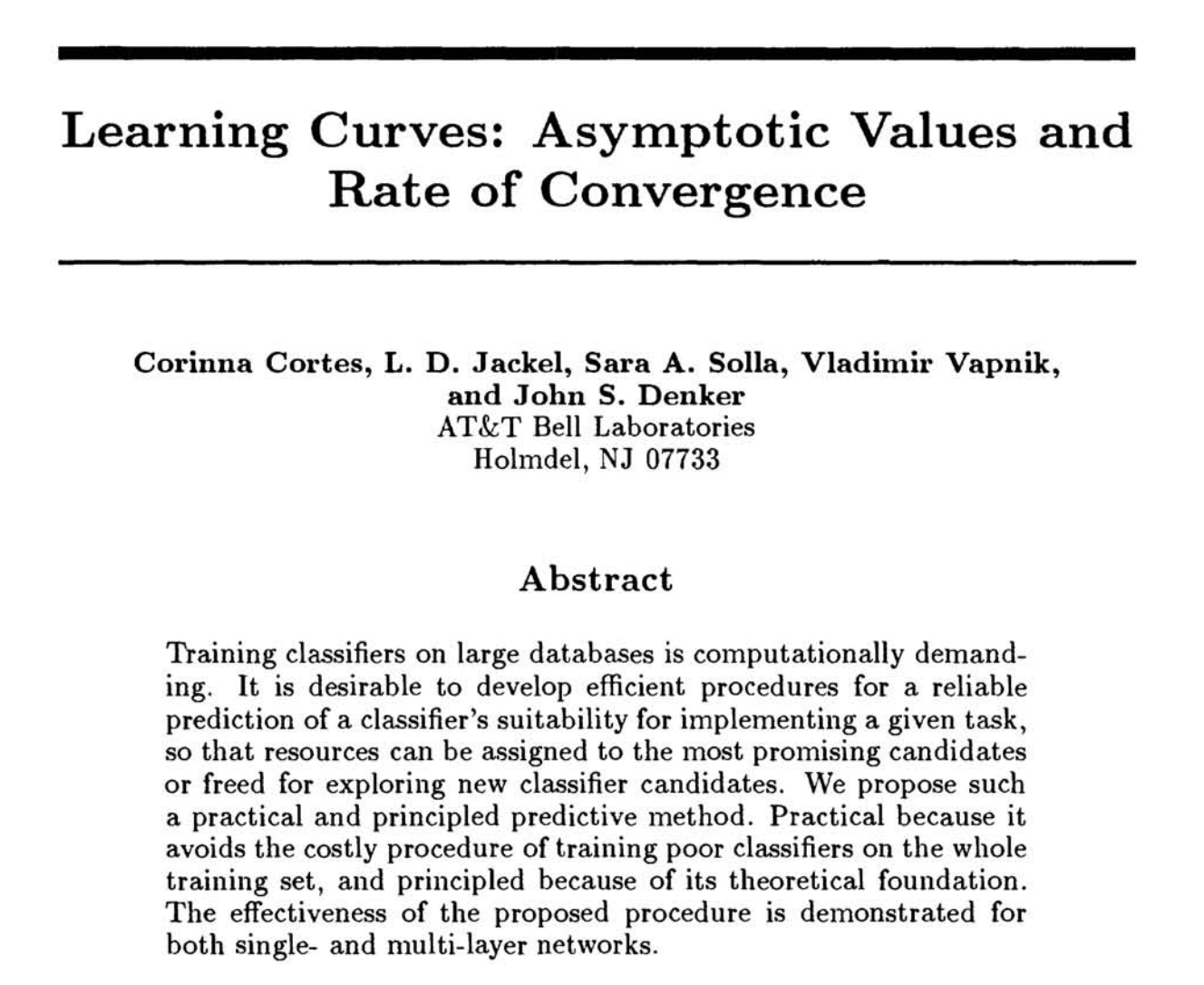
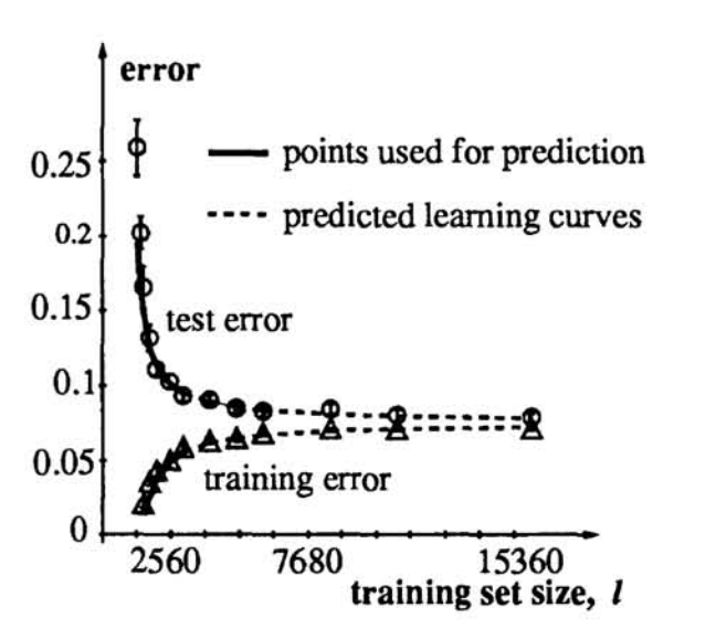
Figure 9.1 Early Bell Labs research on (data) scaling laws

Banko & Brill's classic ACL 2001 NLP paper 《Scaling to Very Very Large Corpora for Natural Language Disambiguation》 pointed out that on certain tasks, increasing data volume brings far greater performance gains than improving algorithms (more data matters more than better algorithms). They plotted log-linear performance curves and proposed a still-influential viewpoint: we should weigh investment in "algorithm R&D" against "data collection."

Confusion Set Disambiguation is an NLP task that aims to select the correct word from a set of easily confused candidates based on context. Example: Confusion set: {to, two, too} Sentence: "I am going ___ the store." Task: The model must determine from context that "to" should be filled in, not "two" or "too."

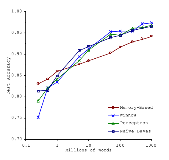
Figure 9.2 Learning curves on confusion set disambiguation tasks

Kolachina et al. (ACL 2012) 《Prediction of Learning Curves in Machine Translation》 validated that predictable mathematical relationships (particularly power-law relationships) exist between "data volume" and "model performance." The research team used the then-mainstream Moses statistical machine translation system, conducting large-scale experiments across 30 different language-pair and domain combinations (e.g., English-German, English-Spanish news, etc.). They tried fitting the relationship between "training data volume (x)" and "translation quality (y, BLEU score)" using different mathematical formulas:

Exponential family: $Ex{p}_3$, $Ex{p}_4$, $Exp{P}_4$ Power-law family: $Po{w}_3$, $Po{w}_4$ Logarithmic family: $ILog2$

Key conclusions from the paper:

• Power Law fits best. The parametric power-law function (Pow3) typically most accurately describes the learning curves of machine translation systems. This means that as long as data continues to increase, model performance will keep improving — refuting the pessimistic assumption that "performance saturates quickly."
• Performance is predictable. With very little parallel data (e.g., 10,000 sentence pairs), their method could control prediction error within 1.5 BLEU. Even without any parallel data at all, merely by analyzing monolingual data features (such as morphological complexity), they could roughly predict the shape of the learning curve.

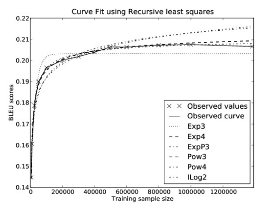
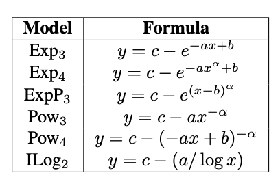
Figure 9.3 Curve fitting on test datasets using different curve families

Hestness et al. (2017) 《Deep Learning Scaling is Predictable, Empirically》 conducted the earliest large-scale neural network scaling law research. They found that across multiple tasks (machine translation, language modeling, speech recognition), model performance follows a predictable power-law relationship. They proposed the famous "three-phase" learning curve: small data region (performance near random guessing), power-law region (stable improvement), and irreducible error region (performance bottleneck).

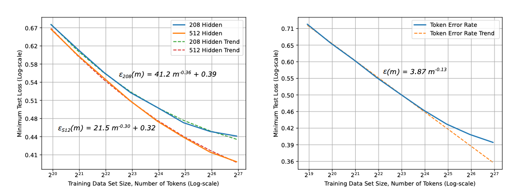
Figure 9.4 Neural machine translation learning curve

Tatsu mentions this paper every time he teaches scaling laws: "Hestness et al. 2017 is the true origin of neural scaling, but they didn't get the citations they deserved. This work was remarkably超前 — they established scaling laws across multiple domains (MT, LM, Speech) and hypothesized the shape of scaling." And with incredible foresight, it already foreshadowed key concepts of the modern LLM era such as "emergence," "compute scaling," and "performance-precision trade-offs."

Figure 9.5 Key concepts proposed by Hestness (2017)

"In 2017, we could already see almost all the phenomena we discuss today. If we had seriously read and thought about this paper back then, we might have understood this entire era much earlier."

9.3 LLM Scaling Behavior

When scaling dataset size or parameters, we always assume the other variable is at saturation. For example, if scaling dataset size, the model size must be far larger than what the dataset size can saturate. Because if data volume far exceeds parameter count, we'll eventually reach saturation (asymptote), but we try to avoid approaching the asymptote.

OpenAI's 《Scaling Laws for Neural Language Models》 found that language model performance has power-law relationships with compute (C), model parameters (N), and dataset size (D).

Figure 9.6 Language modeling performance steadily improves as model scale, dataset size, and training compute increase

We typically assume training and test data follow the same distribution. But even when training and test data come from different sources (e.g., training on Common Crawl, testing on Wikipedia), scaling laws still hold.

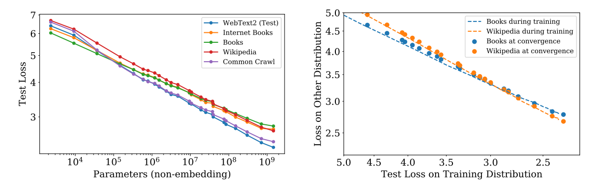
Figure 9.7 Scaling laws when training and test data come from different sources

9.3.1 Data vs. Performance

When we talk about data scaling laws, we mean there is some simple formula mapping dataset size (n) to excess error.

Excess Error is the difference between your current model's generalization error and the minimum possible generalization error achievable by the theoretically optimal model (or Bayes-optimal model). Excess error measures the portion of error that you can "improve" through better algorithms, more data, and better models — as opposed to the irreducible error that cannot be eliminated by improving the model or adding more data.

The learning curve has three phases:

• Best Guess Error: Model performance equals "random guessing" (e.g., in a classification task, always predicting the most frequent class). In this phase, adding small amounts of data barely helps.
• Power-law Region: Exponential increases in data volume bring linear decreases in error. As long as you're in this region, piling on data steadily improves performance.
• Irreducible Error Region: No matter how much more data you add, error won't decrease further. This is due to noise in the data itself (e.g., blurry images, labeling errors) — called Bayes Error; or insufficient model capacity (model is too small to learn more).

We primarily focus on the region from the power-law region to the irreducible error region — it helps us determine whether our model is currently "data-starved" (Phase 2) or has already hit the "ceiling" (Phase 3).

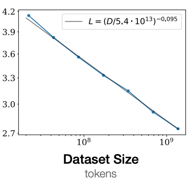
Figure 9.9 Power-law relationship between data size and model error

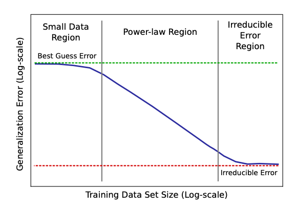
Figure 9.8 Neural machine translation learning curve

An empirical observation: plotting dataset size on the x-axis and model error (Test Loss) on the y-axis, on a log-log plot, they appear as a straight line. Mathematically, a straight line on a log-log plot means there exists a power law relationship between the two variables.

Log-log plot: A special type of chart where both the x-axis and y-axis scales are arranged exponentially, like ${10}^1,{10}^2,{10}^3...$. This type of chart is specifically used to detect power-law relationships.

The x-axis represents the amount of data used to train the model (number of tokens), and the y-axis represents the model's loss on the test set. Lower Loss means the model predicts more accurately and performs better. Blue points are actual experimental data; the gray line is the fitted straight line.

We expect error to be monotonic — with more training data, error decreases. But we don't know the precise functional form. When we say it's a power law, we mean it's linear in log space. If a relationship is linear in log coordinates, it means there exists a polynomial expressing the relationship between the x-axis and y-axis. But why polynomial? Let's answer through two examples.

Example 1: Mean Estimation

Suppose we have data points $x_1,...,x_n$ from a normal distribution $N(\mu ,{\sigma }^2)$. Our task is to estimate the true mean $\mu$ by computing the sample average $\hat{\mu }=\frac{\mathrm{\Sigma }{x}_i}{n}$. The mean squared error is: $\mathbb{E}[(\hat{\mu }-\mu {)}^2]=\frac{{\sigma }^2}{n}$. Error is inversely proportional to sample size $n$. Taking the log: $\log (Error)=-\log (n)+2\log (\sigma )$ — a straight line with slope $-1$.

For neural networks, scaling exponents are much smaller: machine translation is -0.13, speech is -0.3, language models are -0.095. These are much slower than the $1/n$ rate. Why?

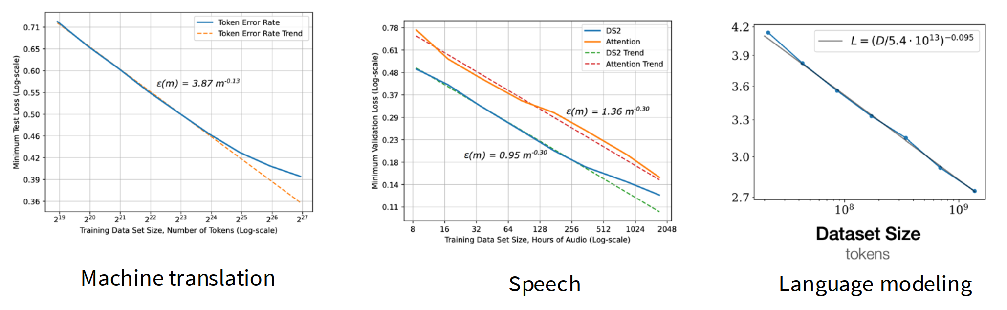
Figure 9.10 Scaling exponents for three different tasks

Neural networks are non-parametric models — they can fit arbitrarily complex functions. For a $d$-dimensional non-parametric learning problem, the error decay rate is approximately $n^{-1/d}$. This means the scaling law exponent $\alpha$ reflects the "intrinsic dimension" of the data manifold. The smaller the exponent, the higher the intrinsic dimension, and the harder the learning task.

"Non-parametric" here doesn't mean there are no parameters, but rather that the number of parameters is not fixed — or the model's complexity can grow无限 as the data volume increases.

Example 2: 2D Prediction Task

In a 2D unit box with $n$ uniformly distributed points, we want to predict the target function $f(x)$. The true value $y$ contains noise $N(0,1)$. Since we don't know what $f(x)$ looks like (non-parametric), the simplest yet most effective method is the "grid-slicing" (histogram method). We slice the 2D plane into many small squares, with side length set to $n^{-1/4}$.

Why slice this way? There's an implicit Bias-Variance Tradeoff here:

• Squares too small: Too few samples fall into each square, causing the computed average to fluctuate wildly (high variance).
• Squares too large: The function varies too much within the square, so representing the entire square with one average is inaccurate (high bias).

Therefore, we take the optimal balance point, giving the optimal side length $n^{-1/4}$.

Side length is $n^{-1/4}$, 2D area is $(n^{-1/4}{)}^2=n^{-1/2}=1/\sqrt{n}$, total area is 1, so total square count is $\sqrt{n}$. Total samples $n$ divided by square count $\sqrt{n}$ equals $\sqrt{n}$. That means each square contains on average $\sqrt{n}$ samples.

Statistics tells us: using $k$ samples to estimate the mean, error (variance) is proportional to $1/k$. Here $k=\sqrt{n}$. So Error $\approx 1/\sqrt{n}$.

If not 2D but $d$-dimensional space, the above logic still holds — only the exponent changes. In 2D, error is $n^{-1/2}$; in $d$ dimensions, the error formula generalizes to: $Error=n^{-1/d}$.

Taking log of the formula above (plotting on a log-log plot): $\log (Error)=-\frac{1}{d}\log (n)$. Let $y=\log (Error)$, $x=\log (n)$. This gives the line equation: $y=-\frac{1}{d}x+C$.

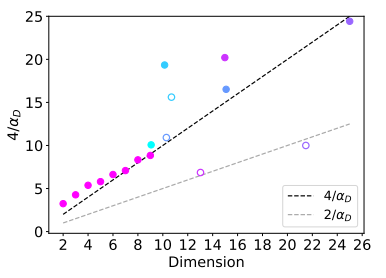
Figure 9.11 Relationship between dimension and scaling law slope

Bahri et al. (2021) attempted to demonstrate through experimental data that the scaling law slope $\alpha$ is indeed determined by the data's intrinsic dimension $d$.

The pink points (Teacher-Student) in the figure are synthetically generated data. We can see they fall perfectly on a straight line (black dashed line). This proves that in theoretically controlled experiments, the Scaling Law's slope is indeed strictly determined by dimension. Other colored points (Real Datasets) represent real-world image datasets (like CIFAR-10, MNIST). Interestingly, they also roughly align along the line (though with some deviation, falling near the gray dashed line).

This strongly supports the "intrinsic dimension theory." It shows that whether artificial or real data, the higher the data's intrinsic dimension (further right on the x-axis), the smaller the Scaling Law slope $\alpha$ (larger y-axis value, since it's the reciprocal), and the harder the model is to train.

However, intrinsic dimension estimation methods are very unreliable, so this conclusion is not airtight. For complex data like "cat photos" or "Shakespeare's text," we actually cannot precisely compute what its intrinsic dimension really is. Current estimation algorithms (Estimators) often have large errors and unstable results. Therefore, while the chart shows correlation, this may partially be because our chosen estimation method happened to match the theory. We cannot yet be 100% certain that Scaling Laws are entirely determined solely by intrinsic dimension.

Data Composition and Scaling Laws

OpenAI's scaling laws paper found that dataset composition only affects the offset (intercept), not the slope. This means you can conduct data selection experiments on much smaller models rather than training at massive scale.

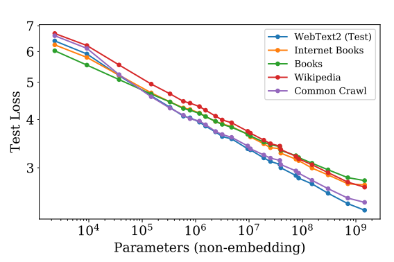
Figure 9.12 Data composition only affects the offset

Hashimoto (2021) in Model Performance Scaling with Multiple Data Sources systematically studied how data composition affects scaling laws.

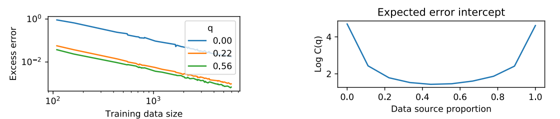
Figure 9.13 How data mixing ratios affect scaling laws

In the left figure, three lines represent three different data mixing ratios $q$ (e.g., $q=0$ means all data from source A, $q=0.56$ means mixed with source B). Regardless of $q$, these three lines have the same slope. This means no matter how you mix data, the rate at which the model improves with increasing data volume is unchanged (i.e., exponent $\alpha$ stays constant). Although the slope is the same, the lines' vertical positions (intercept) differ. The orange line ($q=0.22$) is clearly lower than the blue line ($q=0.00$). This means at the same data volume, better data ratios bring lower error.

In the right figure, the x-axis represents the data source ratio $q$ (from 0 to 1), where 0 means only data source A, 1 means only data source B, and 0.5 means half each. When using only a single data source ($q=0$ or $q=1$), the error intercept is highest (worst performance). When $q\approx 0.5$, the curve reaches its lowest point. This means mixing two data sources (diversity) significantly reduces model error.

Summary:

• Exponent $\alpha$ (slope): Determined by model architecture or task intrinsic dimension. Simply changing data mixing ratios cannot change this "learning rate."
• Constant $C$ (intercept): Determined by data quality and ratio. This figure tells us that by optimizing data ratios (e.g., making data more diverse), we can lower the constant $C$.

Data Repetition

In practice, data is finite. What happens when we repeat the same data across multiple epochs?

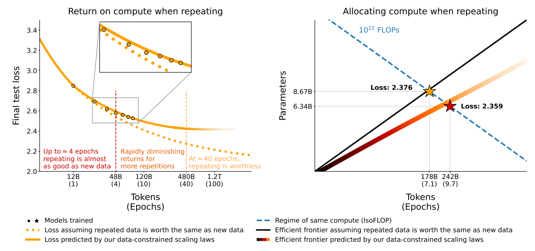
Figure 9.14 Effect of repeated data vs. new data on model performance

Within ~4 epochs, the solid and dashed lines几乎 overlap. This means repeated data in the early stage (within about 4 times) is nearly as effective as new data. Beyond 4 epochs, the solid line begins to明显 deviate from the dashed line — benefits from repeated data rapidly diminish. Around 40 epochs, the solid line完全 flattens. This means repeated data becomes completely worthless — no matter how much more you train, the model learns nothing new, and may even begin to overfit.

The right figure answers: "If I must repeat data, how should I allocate my compute (how big should the model be? how long should I train?)"

The blue dashed line represents a fixed compute budget — any point on this line costs the same money/time. The black solid line assumes the optimal configuration when data is unlimited (Chinchilla Optimal). The red solid line is the optimal configuration when data-constrained (must repeat data). The yellow star (Standard Strategy) recommends training 178B Tokens (7.1 Epochs) with a larger model (8.67B parameters). The red star (Data-Constrained Strategy) recommends training 242B Tokens (9.7 Epochs) with a slightly smaller model (6.34B parameters).

When facing data scarcity and forced to repeat data, to achieve the best results, you should slightly reduce model size and increase training epochs. But even so, the lowest Loss you can achieve (2.359) is only marginally better than the standard strategy (2.376) — it cannot改变 the big picture.

The effective data formula quantifies "how much新 data repeated data is worth":

$$D^{\prime }=U_D+U_D{R}_D^{\ast }(1-e^{\frac{-R_D}{R_D^{\ast }}})$$

$D^{\prime }$ (Effective data) represents the effective data volume — how much knowledge the model feels it has learned; $U_D$ (Unique tokens) is the amount of unique data (original dataset size); $R_D$ (Repetition) is the number of repetitions (Epochs). The first term $U_D$ is the base data volume. The second term contains the $(1-e^{-x})$ form — a classic saturation function. As repetition count $R_D$ increases, this term gradually approaches a constant ceiling. This means no matter how many times you repeat, the effective data volume $D^{\prime }$ has a天花板 and cannot grow infinitely.

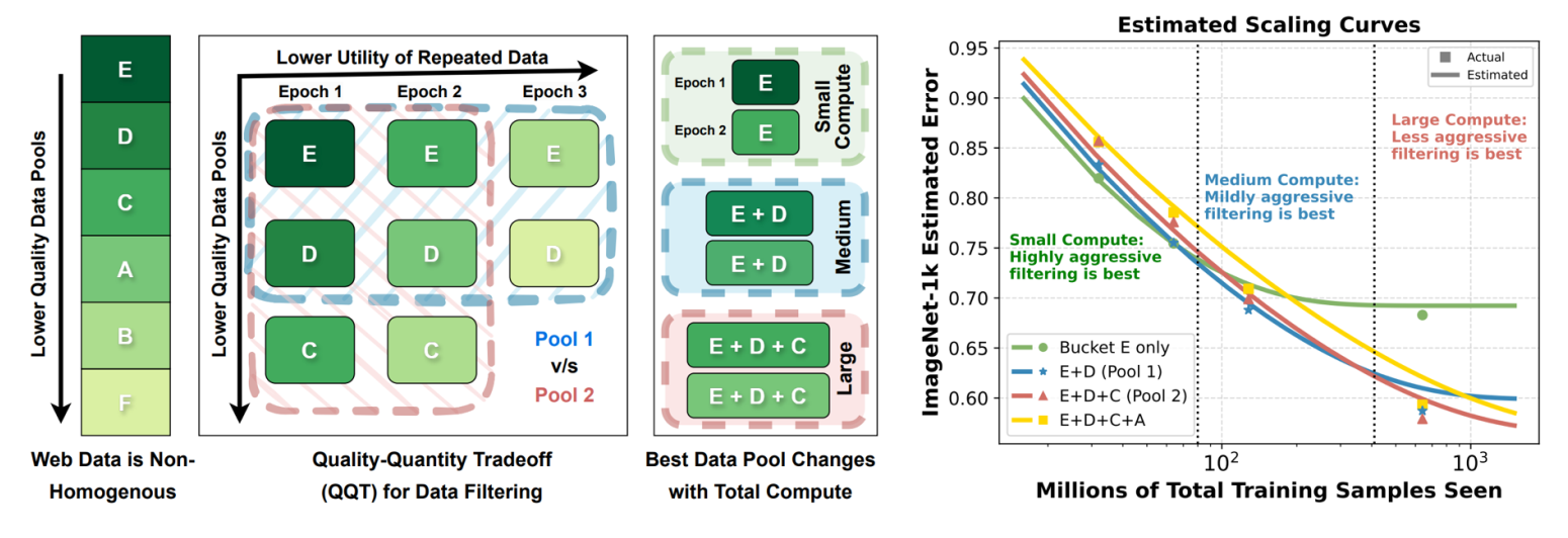
Figure 9.15 Data selection strategy at large scale

If we need to do data selection in a big data environment, which is better: repeating wiki 10 times or including new data? The following study from CMU essentially explores the trade-off between repeating data and selecting lower-quality new data.

In the figure, data quality is divided into different "pools" (Pools): E is the highest, D, C, A, B, F: quality递减 sequentially. The right figure's green line (Bucket E only) uses only the highest quality data; the blue line (E+D) mixes in次优 data; the red/yellow lines (E+D+C) mix in more ordinary data.

The key finding from this research: data selection strategy should change with training scale (compute budget).

• If you're just training a small model (or making a demo), use only the highest quality data — even if数据量 is small, it's fine.
• If you're training a GPT-4 class ultra-large model, overly strict data filtering is actually harmful. You need to relax standards and feed those "decent" data to the model as well, because at large scale, new data matters more than data quality.

---

Review:

• There exists a log-log linear relationship between data and error
• This relationship is robust across different domains and model types
• Using mean estimation as an example provides good theoretical understanding
• Application: data collection / management

---

9.3.2 Model Size vs. Performance

Scaling laws also apply to model size. By comparing scaling curves of different architectures or hyperparameters at small scale, we can predict large-scale performance.

Figure 9.16 Transformer vs. LSTM scaling comparison

Transformer not only outperforms LSTM at the same parameter count, but its scaling curve slope is steeper — meaning the performance gap widens as model size increases.

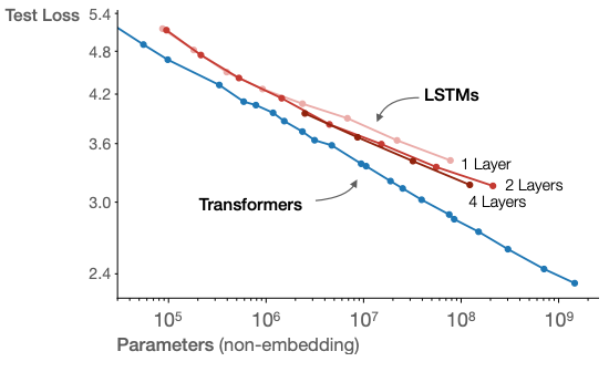
Figure 9.16 Performance comparison of Transformer and LSTM at different parameter scales

Figure 9.17 Compute vs. Performance (FLOPs vs Performance) for different models and architectures

In Scaling Laws vs Model Architectures: How does Inductive Bias Influence Scaling?, researchers compared standard Transformers with various Transformer variants on negative log-perplexity.

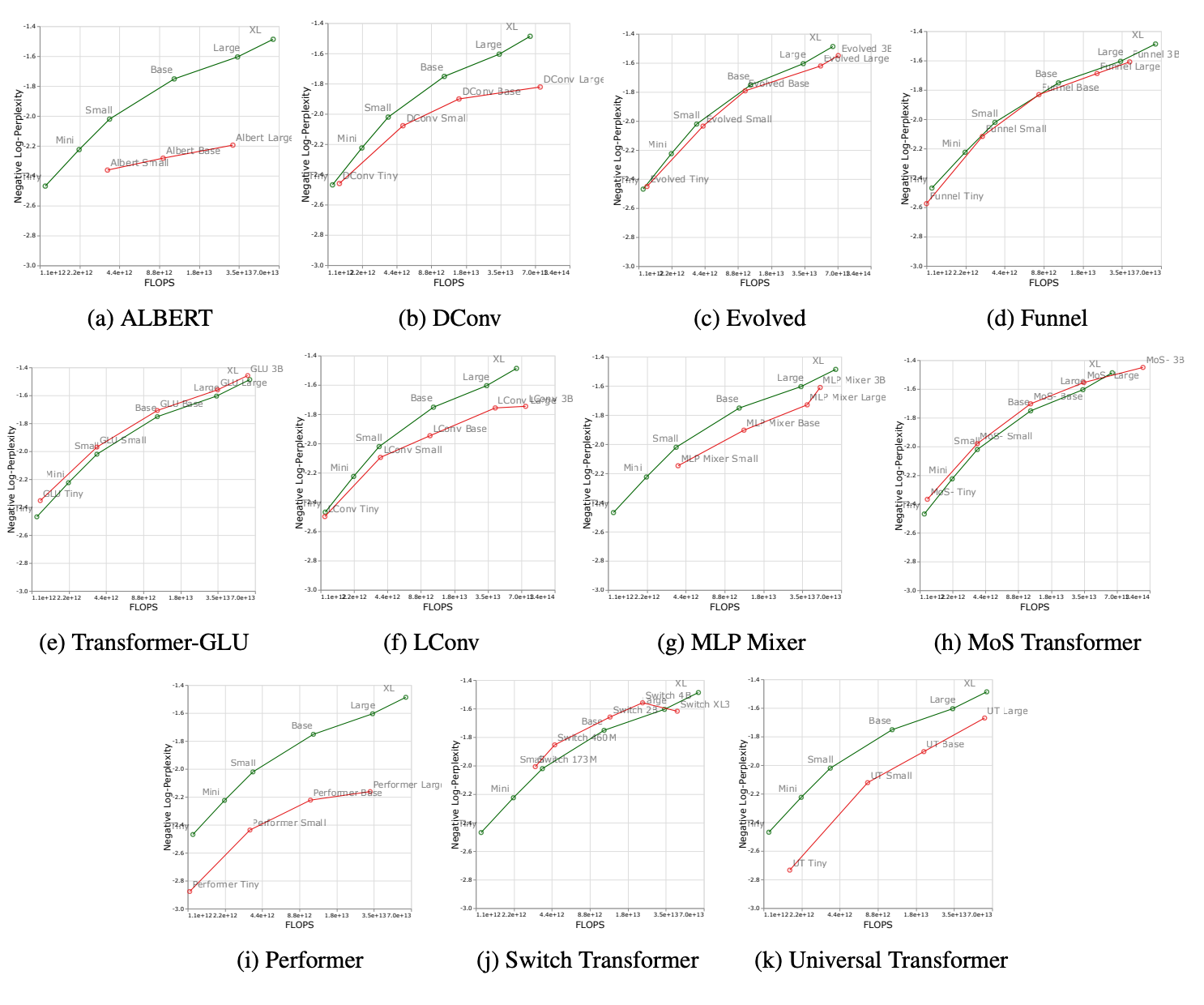
Figure 9.18 Relationship between compute and performance for Transformer and its variants

Green points represent standard Transformers; red points represent specific variants or configurations. Labels (Mini, Small, Base, Large, XL) indicate model sizes. Across Transformer variants, performance (measured by Negative Log-Perplexity) has a strong positive correlation with compute (FLOPs), and this relationship holds universally across different architectures and model sizes.

9.3.3 Hyperparameters vs. Performance

Optimizer Selection: Adam vs SGD

The same methodology can compare optimizers. Experiments show that on RHN (Recurrent Highway Nets), Adam typically has better scaling characteristics (lower curve) than SGD.

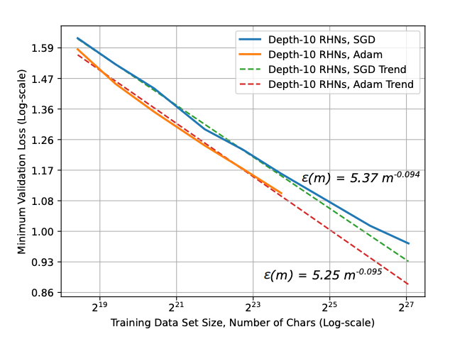
Figure 9.19 Optimizer comparison

Depth/Width: Number of Layers

It's generally believed that deeper layers bring significant improvement. But from the right figure, increasing from 1 to 2 layers brings enormous performance gains. Beyond a certain depth, gains from adding more layers diminish.

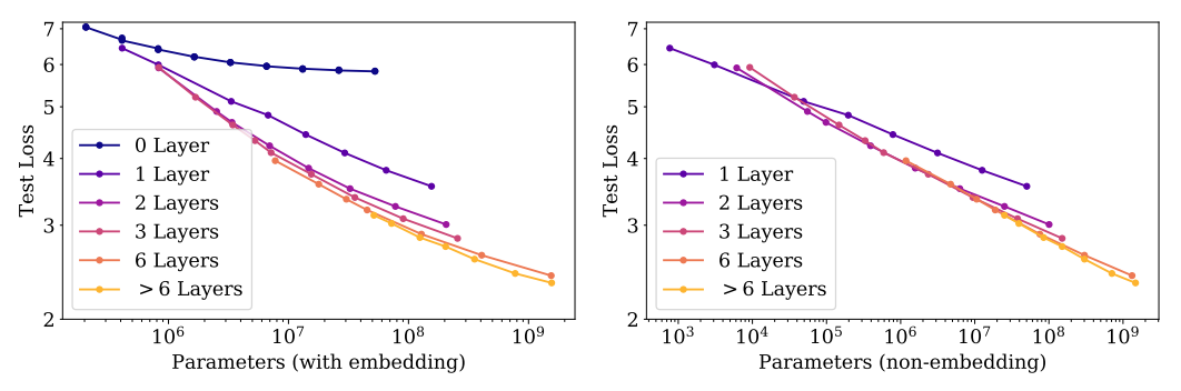
Figure 9.20 Effect of layer count on model performance

Notably, not all parameters produce the same scaling law! If embedding parameters are included as part of the model, the scaling law looks very different (left figure) — it's not a linear relationship.

If embedding parameters are counted, the depth scaling law becomes "very funky-looking." So they decided to exclude all embedding parameters and only count non-embedding parameters. "Because you can convince yourself — embeddings are just table lookups; it's the other parameters that do the computation."

In the figure below, the middle plot's x-axis is the width-to-depth ratio, including not only different model sizes but also different width/depth ratios. Across different x-axis positions, the curve shapes are similar. Performance is optimal between 10~100.

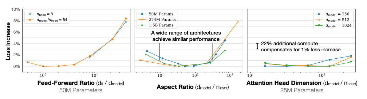
Figure 9.21 Effect of model width and depth on performance

Feed-Forward Ratio $d_{ff}/d_{model}$: the ratio of the Transformer's internal MLP layer width to the model's hidden dimension. Between ${10}^0$ (1) and ${10}^1$ (10), the curve is almost flat. This means whether this ratio is set to 2, 4, or 8, it barely affects model performance. Only when set particularly large (>10), wasting parameters on MLP, does performance degrade.

Aspect Ratio $d_{model}/n_{layer}$: small values mean small $d_{model}$, large $n_{layer}$ — the model is tall and thin (Deep & Narrow). Large values mean large $d_{model}$, small $n_{layer}$ — the model is short and wide. You can train a 48-layer, 1600-dim model or a 6-layer, 4288-dim model. As long as total parameter count is the same, the final Loss differs by less than 3%.

Attention Head Dimension $d_{model}/n_{head}$: the size of each attention head. Whether you set the head size to 64 or 128, as long as total parameter count is unchanged, it barely affects final performance.

Batch Size

Noise scale: the expected gradient noise when randomly sampling within a batch.

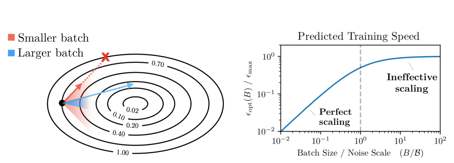
Figure 9.22 Batch size and critical value

When batch size is below the critical value, increasing batch size effectively reduces gradient noise — training speed improves approximately linearly (Perfect Scaling). When batch size exceeds the critical value, returns rapidly diminish (Ineffective Scaling).

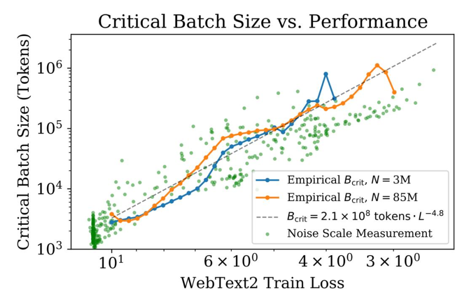
Figure 9.23 Critical batch size and model performance

As you try to reduce loss — moving left to right on the graph (x-axis: 10→6→4→3) — the critical batch size increases, and correspondingly, the overall batch size becomes larger. So, the smaller the target loss, the larger the overall batch size you can use.

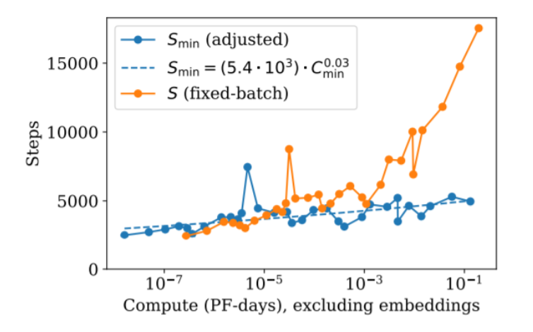
Figure 9.24 Choosing the optimal batch size

As compute and model scale increase, how should we scale training?

• Large batch size, same number of steps
• Fixed batch size, more steps

Learning Rate

When scaling up models, how should the learning rate adjust? Typically, as shown in the left figure below, the optimal learning rate depends on model scale. Larger models generally need smaller optimal learning rates.

μP (Maximal Update Parametrization) (right figure), through a special parameterization and initialization scheme (scale-aware initialization), can keep the optimal learning rate stable across different model scales. This means you can find the optimal learning rate on a small model and directly apply it to train a trillion-parameter model without re-tuning.

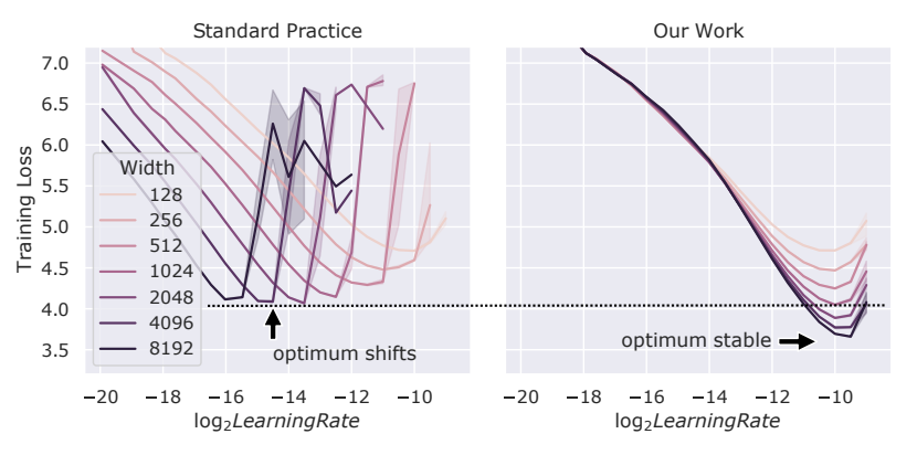
Figure 9.25 Standard approach vs μP improvement

The table below shows how to implement μP. The core idea is adjusting initialization and learning rate based on the model's width scaling factor $r$.

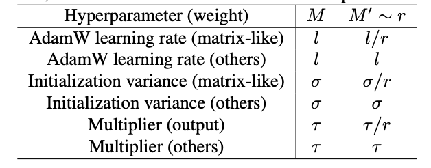
Figure 9.26 Different implementations of μP

Suppose we scale model $M$ to $M^{\prime }$, expanding width by a factor of $r$:

• AdamW Learning Rate (matrix-like): For matrix-type parameters (like weight matrices in Transformers), learning rate needs to be divided by $r$ ($l/r$). This is the most critical step — generally meaning larger models need smaller learning rates.
• Initialization Variance (matrix-like): Initialization variance also needs to be divided by $r$ ($\sigma /r$). This means larger models should have initial weights closer to 0 to prevent signal explosion in deep networks.
• Others: For vector-type parameters (like Bias, LayerNorm), typically unchanged.

In summary, if we simply naively scale up, the optimal learning rate changes, making training difficult. We need a "Scaling Aware" initialization and learning rate strategy (i.e., μP) to keep hyperparameters stable across different model scales.

9.3.4 Scaling Behaves Differently Across Downstream Tasks

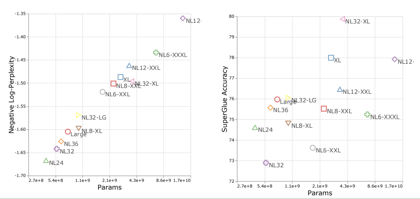
Figure 9.27 Scaling behaves differently across downstream tasks

Left figure: x-axis is compute, y-axis is perplexity, both in log scale. Shows a very good correlation.

Right figure: y-axis is SuperGLUE accuracy — no linear relationship at all. Some models are clearly much better than others.

"This is one of the worst correlations I've seen from upstream to downstream. But it's a very important warning — scaling laws typically only apply on the perplexity side. The transfer from perplexity to downstream is far more uncertain than you might think."

"This is one of the worst correlations I've seen from upstream to downstream. But it's a very important warning — scaling laws typically only apply on the perplexity side. The transfer from perplexity to downstream is far more uncertain than you might think."

9.3.5 Practice Recommendations

Before training, we can effectively select optimizers, model depth, and model architecture. Train small models first, then extrapolate results to predict large model performance.

Steps:

• Train on small models
• Establish some form of scaling law
• Set optimal hyperparameters

9.4 Joint Scaling: Model, Data, and Compute

9.4.1 Joint Scaling Laws

Joint Scaling of Model Size (N) and Data Volume (D)

Under a fixed compute budget, should we train a larger model or use more data to train a smaller model?

To scientifically address this, we need a formula that simultaneously considers both "data volume ($n$)" and "model size ($m$)." This is the joint scaling law. Rosenfeld et al. (2020) and Kaplan et al. (2020) almost simultaneously proposed the joint data-model scaling law:

Figure 9.28 Joint scaling law forms

Rosenfeld et al. (2020) proposed $Error=n^{-\alpha }+m^{-\beta }+C$, which intuitively decomposes error into three parts:

• Error from data ($n^{-\alpha }$): less data → larger this term.
• Error from model ($m^{-\beta }$): smaller model → larger this term.
• Irreducible error ($C$): the task's inherent difficulty baseline.

This means if your model is too small ($m$ very small), the middle term becomes large — no matter how much data ($n$) you add, total error won't come down.

Kaplan et al. (2020) proposed $Error=[m^{-\alpha }+n^{-1}{]}^{\beta }$ — another form from OpenAI, also describing the coupling between model size and data volume, but considering only the reducible error term, hence no constant term $C$.

The figure below shows training on green small data and small models, then extrapolating to red large data and large models:

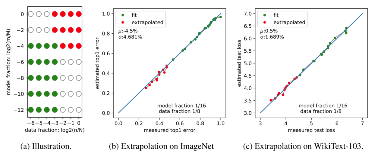
Figure 9.29 Joint scaling of parameters, compute, and data

The x-axis is parameter count, color represents compute, and data volume is the third axis.

Compute vs. Performance Trade-off

This figure (from Kaplan et al. 2020/2021) shows the relationship between model size and performance under different compute budgets.

Left figure: each colored line represents a fixed compute budget. For each fixed compute budget, there exists a unique optimal model size. If you have money, build large models; if you have limited budget, building large models actually performs worse than small ones.

Right figure: small models start with rapidly dropping Loss (fast start), but quickly flatten. Large models start with relatively higher Loss (slow start, because many parameters are hard to train), but as compute investment increases, they overtake small models, and Loss can continue dropping to lower levels.

9.4.2 Chinchilla

DeepMind's Chinchilla paper (Hoffmann et al., 2022), through large-scale experiments, precisely fitted this joint scaling law and arrived at a startling conclusion:

For a given compute budget, model size and data volume should increase in proportion.

Kaplan's original conclusion: $N_{opt}\propto C^{0.73},D_{opt}\propto C^{0.27}$ — tokens per param decreases as compute increases. This means the more compute you have, the more you should train larger models (with relatively less data).

Previous models (like GPT-3) were generally "too large, under-trained." Chinchilla found that to achieve compute-optimality, the ratio of data (tokens) to model parameters should be approximately 20:1.

This means a 70B model (Chinchilla-70B) should be trained with roughly $70B\times 20=1.4T$ tokens, and its performance can exceed a 175B model (GPT-3) trained on less data.

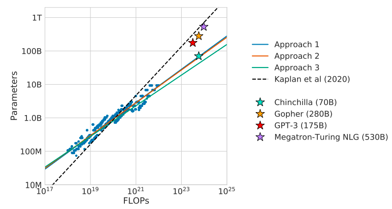
Figure 9.31 Kaplan vs Chinchilla

"I particularly like the Chinchilla paper because it provides three different methods to estimate the data-model tradeoff — a way to robustify oneself against modeling assumptions."

Chinchilla used three methods to find the optimal combination of model size (N) and data volume (D) under a fixed compute budget (FLOPs):

• Minimum over runs: Take the lower envelope of all training curves.
• IsoFLOP analysis: At fixed FLOPs, sweep different N and D combinations to find the performance-optimal point.
• Joint fits: Train models on an N-D grid and directly fit a joint scaling function.

All three methods pointed to the same conclusion: the optimal scaling exponent for both D and N is almost exactly 0.5, meaning the optimal D/N ratio is constant. Chinchilla's specific ratio: approximately 20 tokens per parameter. This means rather than training an enormous model, use the same compute budget to train a smaller but more data-sufficient model — the latter performs better.

9.4.3 Why Do Kaplan and Chinchilla Differ So Much?

Explanation 1: Kaplan excluded embedding parameters (only counting non-embedding params), and at small compute budgets, warmup was too high and learning rate decay may not have been properly tuned. Choosing non-embedding vs. total params changes the parameter counting method, thereby changing the $N_{opt}(C)$ exponent.

Explanation 2: Non-embedding vs. total params choice + small nonlinearities in fitting. Both叠加 produced巨大的 exponent differences.

Interesting footnote — Chinchilla Method 3 had an error (Besiroglu et al. 2024):

"Someone did data forensics — recovered Chinchilla Method 3's original data, re-fitted, and the results matched Methods 1/2. So Method 3's deviation was an error in the original paper."

9.4.4 From Training-Optimal to Inference-Optimal

Chinchilla's law is training-optimal — its goal is obtaining the best-performing model under a fixed training compute budget. But in actual deployment, inference cost dominates the total cost of a model's lifecycle. A smaller model with lower inference cost, even if slightly more expensive to train, may be more economically viable.

Therefore, the industry trend is "over-training" small models — training with data far beyond Chinchilla proportions to换取 stronger inference capability.

Historical trend of actual token/param ratios:

Model	tokens / param
GPT-3	~2
Chinchilla	~20
LLaMA 65B	~22
Llama 2 70B	~29
Mistral 7B	~110
Llama 3 70B	~215

This trend indicates that to reduce inference latency and cost, the industry is willing to invest more compute resources during training to obtain a model that is smaller and more efficient at a given capability level.

Widespread application of IsoFLOP: Not just language models — Diffusion (Gulrajani et al. 2023), MoE (Abnar et al. 2025) all use IsoFLOP to optimize architecture choices.

9.5 Scaling Laws for Diffusion Models

Previously, Scaling Laws were primarily studied on autoregressive models (like GPT-style LLMs). Likelihood-Based Diffusion Language Models studied the validation of scaling laws on Diffusion Models, with the main finding being that diffusion models also follow the same scaling laws.

The "Iso" prefix means "equal" — IsoFLOP is about finding the optimal balance between model size (parameter count) and training data volume under a fixed total compute budget. The left figure shows autoregressive model IsoFLOP curves. The middle figure shows diffusion model IsoFLOP curves. The right figure connects all the "stars" (optimal points) from the left and middle figures — on a log-log plot, these optimal points form a straight line, meaning diffusion models also strictly follow power laws. As long as we increase compute, we can precisely predict how well diffusion models will perform.

9.6 Case Studies and Implementation Details of Scaling

As LLMs enter the production era, the industry has become increasingly cautious about disclosing core scaling strategies (such as data-model trade-offs, hyperparameter selection). Therefore, we can only glimpse their internal logic through a few publicly available, detailed research cases. This section will deeply analyze three exemplars: Cerebras-GPT, MiniCPM, and DeepSeek, enabling readers to understand how developers of modern top-tier language models actually use scaling laws to design and optimize their models.

9.6.1 Cerebras-GPT

Cerebras-GPT followed Chinchilla scaling laws (20 tokens per parameter), training 7 GPT-3-style models from 0.1B to 13B. It was the first to publicly validate the effectiveness of muP (Maximal Update Parametrization) in large model scaling.

• Models using muP exhibit more stable scaling behavior

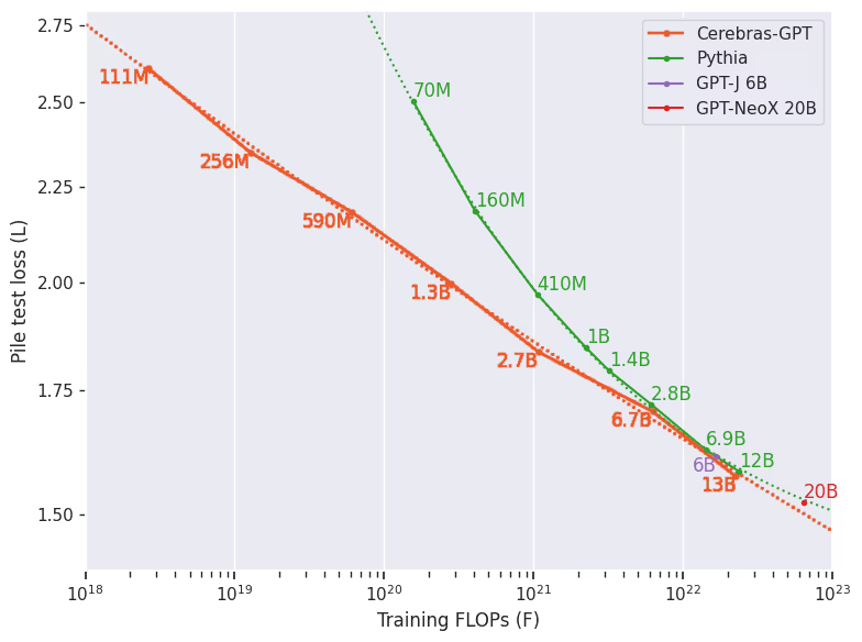
Figure 9.34 muP demonstrates more stable scaling laws

• Using muP brings more predictable scaling

Researchers first trained a small model (10M parameters) using muP scaling laws, then transferred these hyperparameters to larger Cerebras-GPT models.

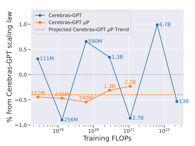
Figure 9.35 muP demonstrates more predictable scaling laws

The paper's appendix also provides detailed implementation comparisons between Standard Parameterization (SP) and muP:

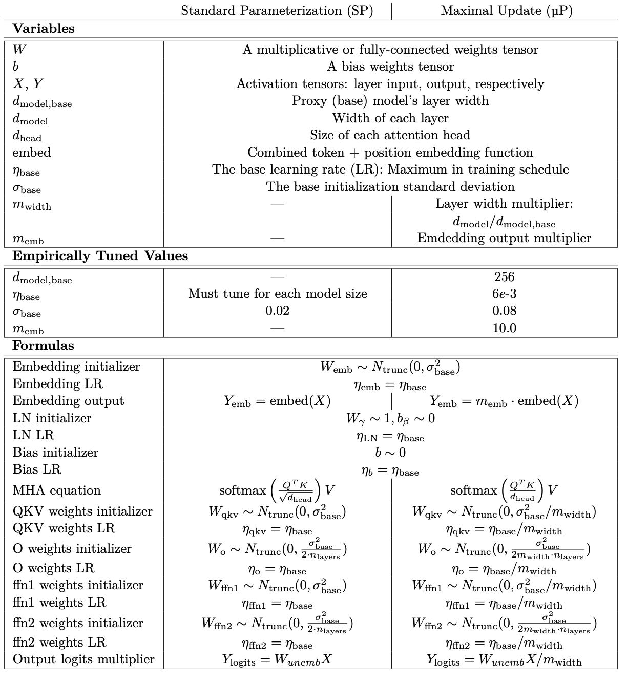
Figure 9.36 Detailed implementation comparison of SP and muP

Showing how the Cerebras team found optimal hyperparameters for their μP models. The core idea is "µTransfer": find a good set of hyperparameters on a small model, then directly apply them to large models without needing to re-tune for each large model.

Random hyperparameter search on three key hyperparameters using a 40M parameter small model:

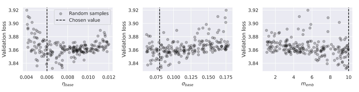
Figure 9.37 Random hyperparameter search on three key hyperparameters using a small model

Left: η_base (base learning rate); Middle: σ_base (base weight initialization std); Right: m_emb (embedding scaling factor). Final determined hyperparameters: η_base = 6e-3, σ_base = 0.08, m_emb = 10.

Through a one-time search on a small model, hyperparameters applicable to large models were obtained, dramatically simplifying the large model training pipeline and reducing cost and complexity.

9.6.2 MiniCPM

MiniCPM is a series of LLMs launched by ModelBest, a startup spun out of Tsinghua's NLP lab — one of the earliest teams in China to develop LLMs, with strong capabilities and a unique technical approach. Notably, in June 2025, when a Stanford student AI team's open-source multimodal model was rumored to have "wrapped" ModelBest's MiniCPM-Llama3-V2.5, this Tsinghua-affiliated LLM startup再次 received public attention. Their current development path focuses more on on-device models, carving out a distinctive path.

When they launched the MiniCPM model in 2024, it ranked among the top tier of open-source models, beating many 7B-scale models with a smaller 2B model.

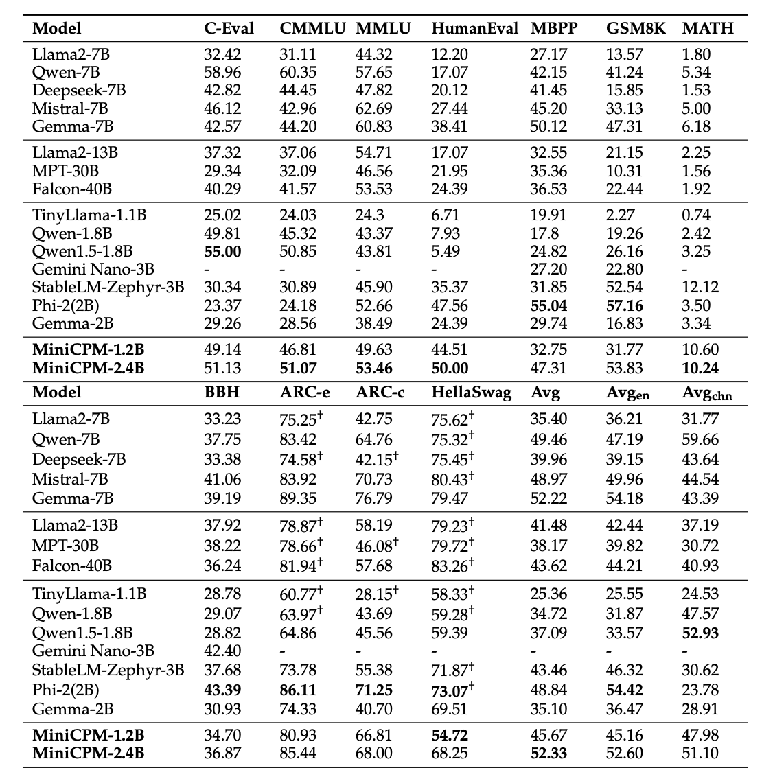
Figure 9.38 MiniCPM performance comparison with other SOTA models

MiniCPM Also Uses muP for Stable Scaling

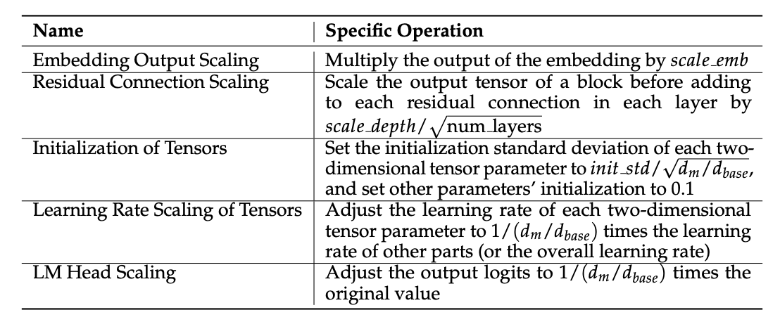
Figure 9.39 Stable scaling with muP

• MiniCPM results: Scale_emb = 12, scale_depth = 1.4, init_std = 0.1, lr = 0.01
• CerebrasGPT results: Scale_emb = 10, lr = 6e-3, init_base = 0.08

We find MiniCPM and CerebrasGPT obtained the same type of scaled embeddings, similar learning rates (roughly 2× difference). Overall, they achieved similar results in hyperparameters.

MiniCPM Model Scaling Strategy

The MiniCPM project's model scaling strategy used during "Model Wind Tunnel Experiments" can be summarized in three points:

• Use μP to initialize model parameters: This ensures that regardless of model size changes, internal structure and hyperparameters (especially learning rate) remain stable, enabling fair comparison of different-scale model performance.
• Fix the aspect ratio: "Aspect ratio" here means the ratio of model architecture "depth" to "width." Specifically, keep the relative proportion between d_m (model hidden dimension) and L (number of layers) roughly constant. This isolates variables, ensuring performance differences are primarily caused by model scale (parameter count) changes rather than fundamental architectural shape changes.
• Scale up overall model size: Gradually build models from 9M to 500M parameters by increasing N(B) (non-embedding parameters), d_m, L, etc.

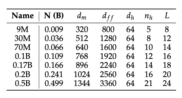
Figure 9.40 Model and training configurations in scaling curves

The largest model in this table is 0.5B (500M) parameters. But the最终 released MiniCPM main models (like 1.2B and 2.4B) are much larger — roughly 5× this maximum experimental model. This shows the authors first conducted exhaustive "wind tunnel experiments" with a series of small models (9M-500M), found the optimal hyperparameters and scaling rules (like μP), and then directly applied this successful experience to the larger 1.2B and 2.4B models, avoiding expensive and time-consuming blind hyperparameter tuning for large models.

They didn't do separate grid searches for each large model. Instead, by analyzing training data from these small models (9M-500M), they fitted optimal batch sizes, learning rates, and data-to-model-size ratios (token-to-size ratios). Then, these empirically-derived formulas from "scaling analysis" were directly applied to the 1.2B and 2.4B large models.

Optimal Batch Size

Shows training loss for three different-scale models (9M, 30M, 170M params) under different data volumes and batch size combinations.

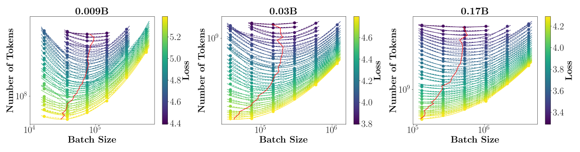
Figure 9.41 Training loss curves for three different-scale models using different batch sizes

X-axis (Batch Size); Y-axis (total processed tokens, representing training progress or compute); each vertically arranged column of points represents a fixed batch size's loss curve as training progresses (Y-axis increases); the red curve connects the batch size achieving the lowest loss at each specific data volume (Y-axis value) — i.e., the "optimal batch size" trajectory.

From the three sub-figures, regardless of model size (9M, 30M, 170M), a clear red curve exists. This indicates that for any given training data volume, an optimal batch size exists that enables the model to achieve optimal performance at that data volume. This optimal batch size increases as training data volume increases.

Then, connecting these three lines, we find they connect well in log space as a linear relationship, yielding the following relationship between batch size bs and C4 loss L:

$$bs=\frac{1.21\times {10}^9}{L^{6.24}}$$

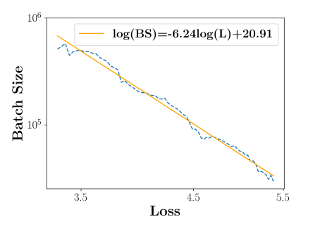
Figure 9.42 Connecting optimal batch sizes

To achieve lower loss (better performance), larger batch sizes are needed.

Optimal Learning Rate

According to muP theory, when model scale expands, the optimal learning rate should remain stable. Does this theory hold in practice?

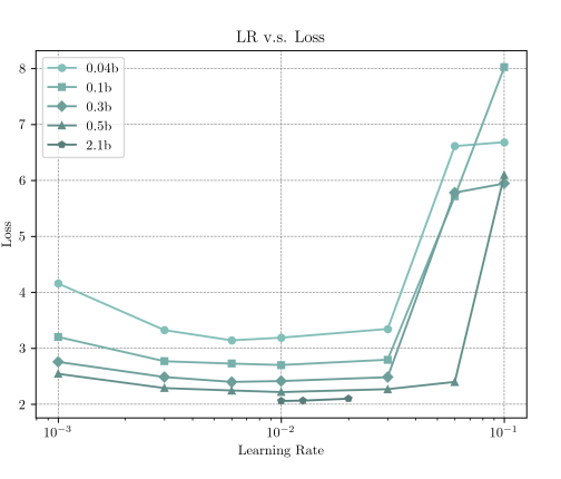
Figure 9.43 MiniCPM maintains learning rate stability using muP

From 0.04B to 2.1B (50× growth), the "lowest point" (optimal learning rate) for all different-scale models clusters around 0.01. This result perfectly validates muP's learning rate stability.

How to Efficiently Study the Scaling Relationship Between Model Size and Data Volume?

To precisely fit a scaling law, each model size and data volume combination must be trained from scratch once. With m model sizes and n data volumes, this requires O(mn) complete training experiments — prohibitively expensive in resources, nearly infeasible for large model training. So how can we avoid this?

To solve the early-stopping problem in Chinchilla analysis, they introduced WSD (Warmup-Stable-Decay) learning rate scheduling.

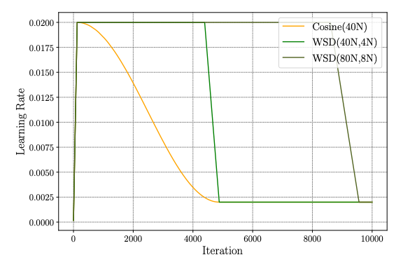
Figure 9.44 Learning rate strategy comparison

WSD consists of three phases: Warmup, Stable, and Decay. The two WSD curves in the figure (WSD(40N,4N) and WSD(80N,8N)) share the same stable training phase. This means you can, after a long stable phase (e.g., 80N steps) of training, start from any intermediate checkpoint (e.g., 40N steps) and仅 perform a short decay (e.g., 4N steps) to obtain an excellently performing model. This allows approximating training results under different data volumes from a single complete training run by performing decay at different points in the stable phase, dramatically reducing the computational cost of Chinchilla-style analysis.

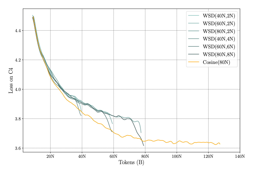
Figure 9.45 Model training loss suddenly drops during WSD's decay phase

The actual behavior of model loss (Loss) as a function of processed token count when training with WSD: slow decline during the stable phase, but during the decay phase, model loss急剧 drops, reaching or even exceeding traditional Cosine's final loss level in a very short time; the decay phase typically only needs ~10% of total training steps (e.g., in WSD(80N,8N), 8N is 10% of 80N) to achieve a performance leap.

Combining WSD and multi-scale training, they used Chinchilla Method 1 (lower envelope) and Method 3 (joint fitting) to determine the optimal data-model ratio. They arrived at an extremely high ratio (~192 tokens/param), suggesting that through fine-tuning, we can significantly超越 the early Chinchilla baseline (20 tokens/param).

Other Methods for Estimating Chinchilla Curves

Gadre et al., in Language models scale reliably with over-training and on downstream tasks, proposed a fitting-curve-based method for estimating Chinchilla curves.

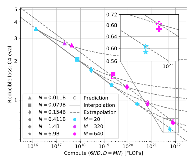
Figure 9.46 Validation loss vs. compute relationship

Core idea: "the 'penalty' from over-training is stable." This means when a model is trained to optimal loss under a given compute budget, its performance bottleneck is primarily determined by model size and data volume, not by insufficient training.

The classic formula for fitting scaling laws is given below:

$$L(N,D)=E+A{N}^{-\alpha }+B{D}^{-\beta }$$

This is the通用 form describing the relationship between model loss L, model parameter count N, and training data volume D.

• E: A base constant term in the loss, representing the theoretical lower bound of model capability or the "irreducible loss" that cannot be eliminated by increasing parameters or data.
• $A{N}^{-\alpha }$: Represents loss due to insufficient model size. A is a fitting constant, α is the model scale scaling exponent. As N increases, this term decreases, indicating larger models better capture patterns in data.
• $B{D}^{-\beta }$: Represents loss due to insufficient data volume. B is a fitting constant, β is the data volume scaling exponent. As D increases, this term decreases, indicating more data enables the model to learn richer knowledge.

Hoffmann et al. (2022), by fitting大量 experimental data, found that α and β values are very close (approximately 0.35), meaning to achieve optimal performance, model parameters N and data volume D should grow at the same rate.

The formula below is a mathematical transformation of the above, re-expressing loss L as a function of total compute C and data-model ratio M. This is for more intuitive analysis of how to allocate resources (i.e., choose model size and data volume) under a fixed compute budget to achieve optimal performance.

$$L(C,M)=E+(a{M}^{\eta }+b{M}^{-\eta })C^{-\eta }$$

• C: Total compute (FLOPs), approximated as C = 6ND.
• M: Data-model ratio (Token Multiplier), defined as M = D/N. Larger M means the model is relatively "smaller" compared to data,更容易 overfitting.
• η: New scaling exponent, defined as η = α/2.
• a, b: New fitting constants, calculated from a = A(1/6)^{-η} and b = B(1/6)^{-η}.

Chinchilla-type Analysis

The authors adopted Hoffmann et al. (2022)'s scaling law formula L(N, D) = C_N * N^{-α} + C_D * D^{-β} + L_0 to fit their experimental data. The goal: under fixed total compute C = 6ND, find the optimal model size N_opt and optimal data volume D_opt that minimize loss, and compute their ratio N_opt / D_opt. The formula for computing optimal ratio: N_opt / D_opt = K² * (C/6)^η. This formula shows that the optimal ratio depends on total compute C.

The MiniCPM team chose two methods for analysis: "lower envelope" and "joint fit."

"Lower envelope" means: for each fixed compute budget, select the lowest loss achievable across all different-scale models. The curve connecting these lowest-loss points is the "lower envelope." The figure below shows how loss changes with compute for three different tasks (Code, English Wikihow, Chinese Wikihow).

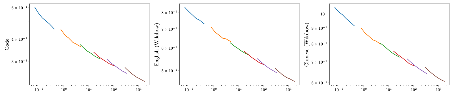
Figure 9.47 Results of scaling experiments using WSD on three tasks

Different colors represent different models. Their results indicate that the diminishing returns effect from data is relatively low. This suggests that at current model scales, increasing data volume can still bring significant performance improvements.

"Joint fit" means treating model size N and data volume D as two independent variables, performing a single global fit across all experimental data points simultaneously to obtain a unified scaling law formula.

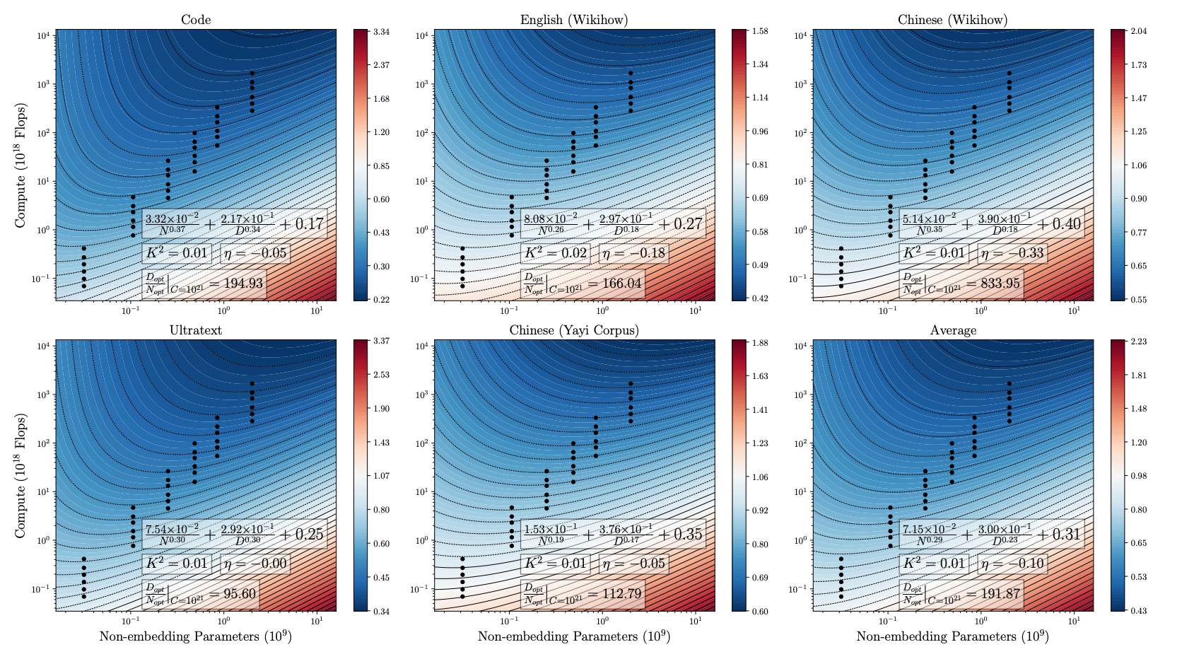
Figure 9.48 Fit results of scaling experiments using WSD on three tasks

The most important result, taking sub-figure 4 as an example: D_opt / N_opt | C=10²¹ = 95.60. This means, under a compute budget of 10²¹ FLOPs, the optimal data volume should be 95.6× the model size. This ratio (~100:1) is far higher than the 20:1 proposed in the Chinchilla study.

Small Models with Lots of Data

Under a given compute budget, to achieve optimal performance, models should be "fed" data at 192× their own parameter count. This number (192) stands in sharp contrast to Hoffmann et al. (2022)'s "20:1" ratio proposed in the Chinchilla study. The authors emphasize that although the trend is consistent (optimal data-model ratio changes as compute increases), the absolute values differ enormously.

This finding was derived from efficient experiments using the WSD scheduler. By training through the stable phase and then仅 using少量 decay steps to evaluate performance under different data volumes, the data axis could be explored at linear cost, ultimately fitting this high ratio. Newer models like LLaMA 3 also adopt higher data-model ratios, indicating that the "20× rule" is merely a rule of thumb — through finer optimization, it can be surpassed.

Scaling Curve Fits Well

The figure contains 12 sub-plots, corresponding to different model sizes (from 0.031B to 2.0B) and different downstream tasks (Code, English (Wikihow)).

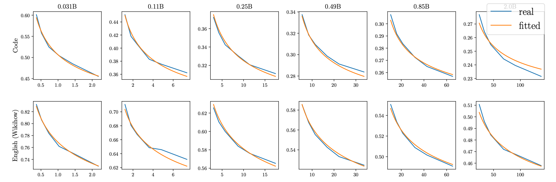
Figure 9.49 Scaling curves using WSD across different model scales and downstream tasks

This proves their method of conducting efficient experiments using the WSD scheduler is reliable, and the collected data is of high quality.

9.6.3 DeepSeek

As DeepSeek's foundational model opening work, DeepSeek LLM: Scaling Open-Source Language Models with Longtermism, officially open-sourced DeepSeek-V1. Although V1's performance wasn't as dazzling as V3, at the time it achieved parity with LLaMA 2 at equivalent scale.

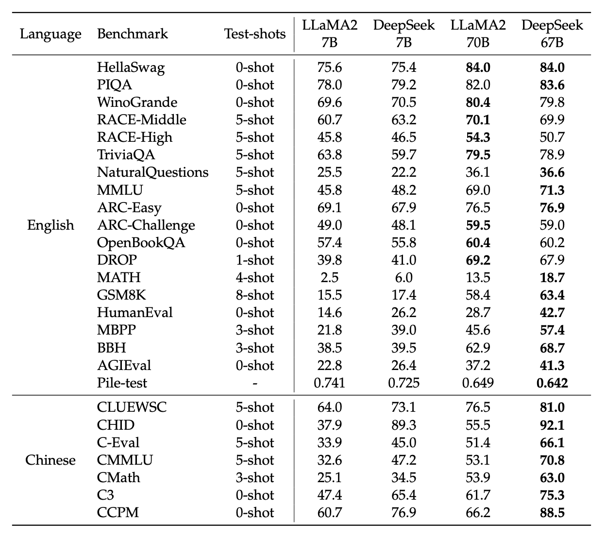
Figure 9.50 DeepSeek performance comparison with other SOTA models

In scaling strategy, DeepSeek represents another pragmatic technical approach — they didn't use muP, but chose to directly fit scaling laws to guide hyperparameter selection.

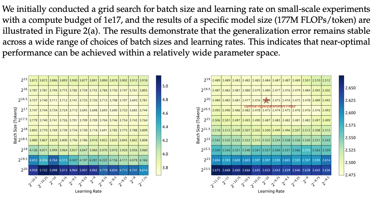
Figure 9.51 Batch size and learning rate combinations under a given budget

This figure aims to empirically study which batch size and learning rate combinations enable the model to achieve optimal or near-optimal performance under a given compute budget. The region with the darkest color and lowest generalization error concentrates in the bottom-right. This indicates that for this specific compute budget and model scale, larger batch sizes and relatively smaller learning rates yield better performance.

This figure shows how DeepSeek LLM's optimal batch size and optimal learning rate change with different compute budgets (Non-Embedding Training FLOPs).

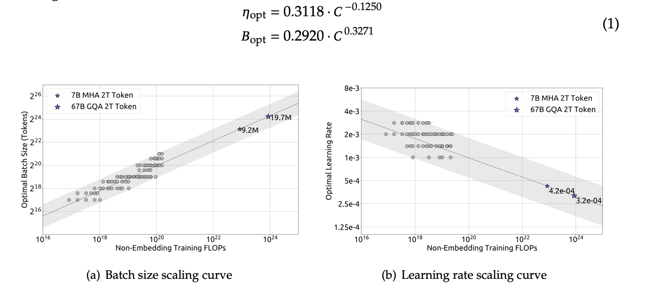
Figure 9.52 Trends of optimal batch size and optimal learning rate under different compute budgets

(a) Batch size scaling curve (b) Learning rate scaling curve. By fitting大量 experimental data, the paper authors determined the power-law relationships between these two key hyperparameters (batch size and learning rate) and training compute budget.

We can see the batch size fitting curve shows a very good linear relationship, but the learning rate fitting curve doesn't appear perfectly linear — data points cluster. The paper describes this as "near-optimal hyperparameters exist in a broad region." The author personally considers this "broad region" as an acknowledgment and "concession" from ideal to reality — it accepts real-world non-perfection.

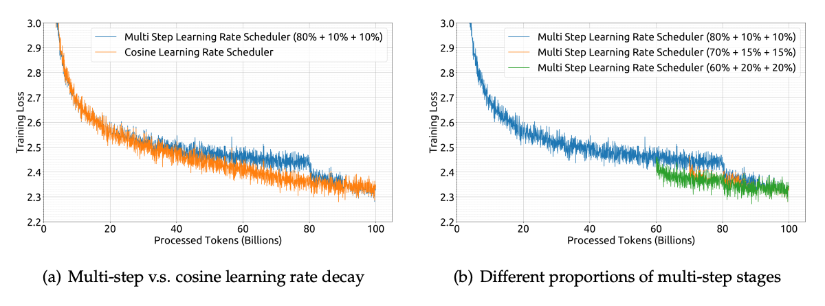
Figure 9.53 Effect of different learning rate schedulers on training loss

Figure (a): Although the two schedulers show slightly different loss decline trends during training, ultimately after processing 100B tokens, their training losses are very close. This indicates multi-step learning rate schedulers remain基本上 consistent with cosine schedulers in final model performance. But an important reason for choosing multi-step schedulers is they're more convenient for "continual training" — i.e., continuing training on an existing model, reusing the first phase's training成果. Meanwhile, they also verified (Figure b) that different phase ratio choices in multi-step schedulers have limited impact on final performance.

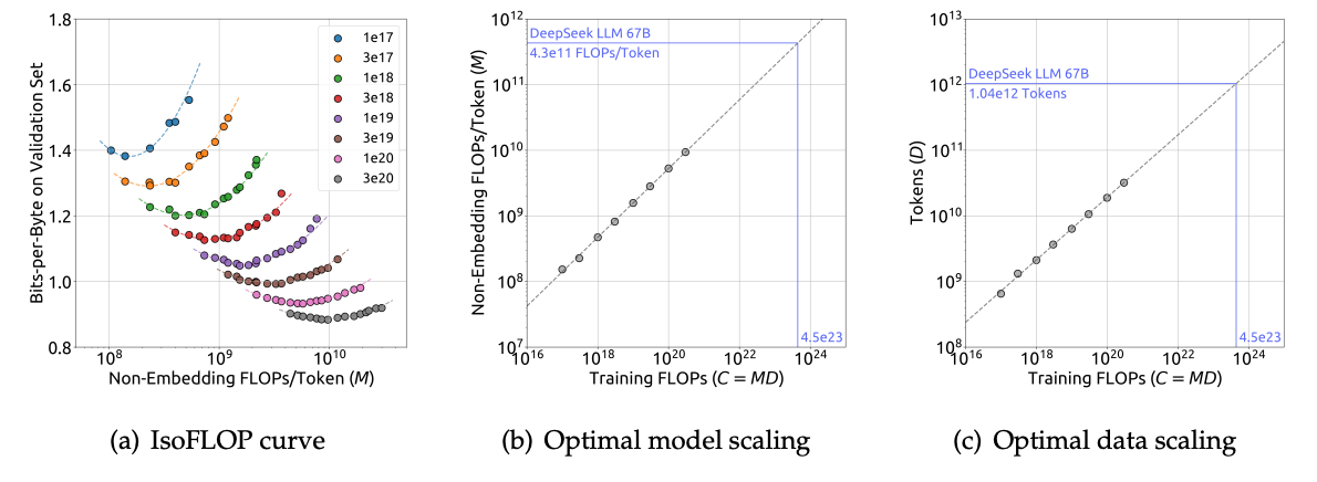
Figure 9.54 Scaling law between compute budget, model scale, and data scale

IsoFLOP analysis = comparing model performance across different (N,D) combinations under the same total compute (FLOPs).

This figure demonstrates the scaling law in LLM training, specifically showing how compute budget (C), model scale (M), and data scale (D) interact, and how to find the optimal model and data allocation strategy to minimize generalization loss. Figure (a): each dashed line represents a fixed total compute budget (C), from 1e17 FLOPs to 3e20 FLOPs. Each point represents the Bits-per-Byte performance corresponding to different model scales (M) under that compute budget. Each curve shows a roughly "U"-shaped trend, indicating that under fixed compute budget, an optimal model scale (M) exists that minimizes Bits-per-Byte (best performance). As compute budget (C) increases (from blue to gray curves), the curve's lowest point (optimal performance point) shifts downward and rightward. This indicates:

• Under larger compute budgets, models can be larger (larger optimal M).
• Under larger compute budgets, models can achieve lower generalization loss (lower minimum Bits-per-Byte), meaning better performance.

Figure (b) reveals the optimal growth path for model scale. The study found that optimal model scale $M_{opt}$ has a power-law relationship with compute budget C: $M_{opt}\propto C^a$, where a is the model scaling exponent. This means as compute resources increase, models should become larger.

Figure (c) reveals the optimal growth path for data scale. The study found that optimal data scale $D_{opt}$ also has a power-law relationship with compute budget C: $D_{opt}\propto C^b$, where b is the data scaling exponent. This means as compute resources increase, the data volume needed for model training should also increase accordingly.

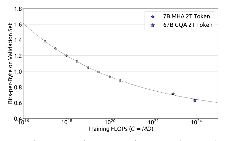
Figure 9.55 DeepSeek's validation set performance under different training compute budgets

This figure shows DeepSeek LLM's validation set performance under different training compute budgets — the so-called "performance scaling curve." It validates that the paper's proposed scaling law can effectively predict large-scale model performance. The key point: DeepSeek LLM 7B and 67B — two large-scale models — have actual performance (blue star points) highly consistent with the scaling curve (dashed line) fitted from small-scale experimental data. This demonstrates that scaling laws obtained from small-scale experiments can accurately predict the performance of large-scale models when compute increases by hundreds or even thousands of times (e.g., experiments at 10²⁰ scale can predict models at 10²³ or 10²⁴ scale). This provides researchers and developers reliable performance expectations and resource allocation optimization guidance before investing enormous compute resources in training large models.

9.6.4 Scaling Laws for Other Models

LLaMA 3 (2024) Scaling Laws

The chart below powerfully demonstrates the Llama 3 team's success in applying scaling laws to model development.

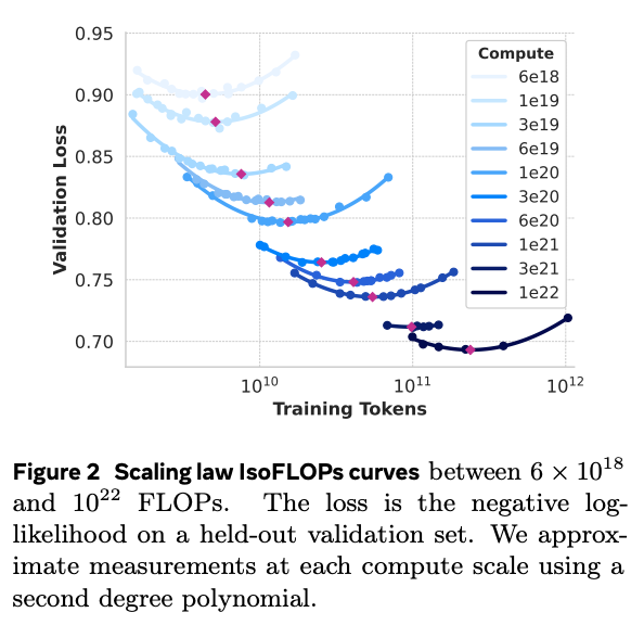
Figure 9.56 Llama 3's IsoFLOPs Scaling Law curves

This figure shows how the Llama 3 team used scaling laws ((39:1 ratio)) to guide pretraining, achieving optimal model performance under different compute budgets.

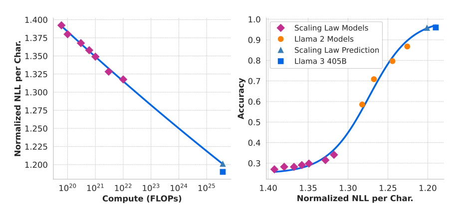
Figure 9.57 Scaling law prediction for ARC-Challenge

This figure shows how the Llama 3 team used scaling laws to predict their model Llama 3 405B's performance on a specific downstream task (here, the ARC Challenge benchmark). Left: compute (FLOPs) vs. normalized negative log-likelihood (NLL); Right: normalized NLL vs. Accuracy.

Hunyuan-1 (2024) Large Scaling Laws

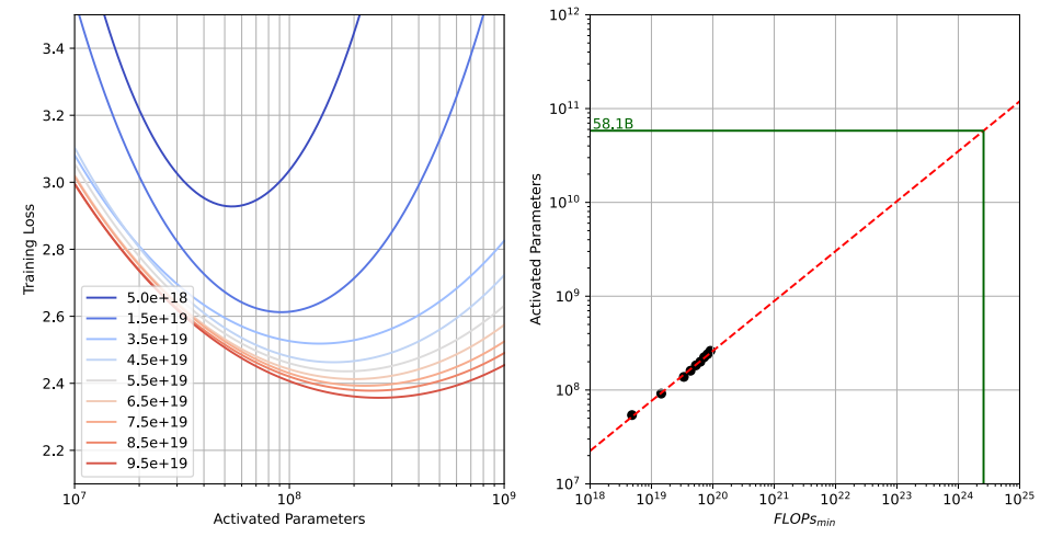
Figure 9.58 Hunyuan MoE model Scaling Law

This figure shows important findings about Mixture of Experts (MoE) model scaling laws during Hunyuan-Large model pretraining. Left: training loss vs. activated parameters under different compute budgets; Right: relationship between activated parameters and minimum compute budget. Additionally, the study指出 that in large language model (especially MoE) pretraining, to achieve compute efficiency optimality, the ideal configuration is approximately 96 training tokens per activated parameter.

MiniMax-01 (2025)

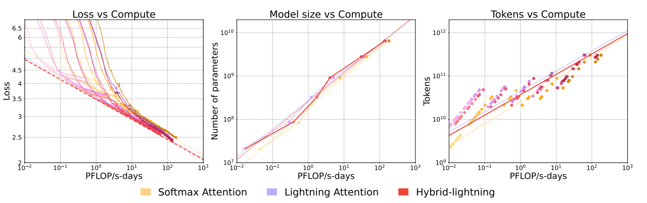
Figure 9.59 MiniMax Scaling Laws

This figure shows how three different attention mechanisms (Softmax Attention, Lightning Attention, Hybrid-lightning) scale in terms of model performance (Loss), model scale (Number of parameters), and training data volume (Tokens) under different compute budgets (in PFLOP/s-days).

MiniMax-01 used their own developed architecture scaling laws for different attention mechanisms, and in determining model scale and training data volume to maximize computational efficiency and performance, they借鉴 the compute-optimality scaling methodology proposed in the Chinchilla paper. This enabled them to balance enormous parameter scale and long-context capability while optimizing the training process, ultimately building the MiniMax-01 series models.

9.6.5 Summary

CerebrasGPT

• Uses muP to keep hyperparameters invariant across model scale changes
• Directly uses Chinchilla scaling formula

DeepSeek

• Assumes most Transformer hyperparameters remain invariant across model scale changes
• Performs scaling analysis on batch size / learning rate to find optimal scaling ratios
• Conducts IsoFLOP analysis to determine model size
  • Uses piecewise linear scheduler to reduce Chinchilla-style scaling cost

MiniCPM

• Uses muP to keep Transformer architecture and learning rate invariant across model scale changes
• Uses piecewise linear scheduler (WSD, Warmup-Stable-Decay) to obtain samples for Chinchilla Method 3 (curve fitting)

LLaMA 3 / Hunyuan

• Only follows IsoFLOP principle, no other detailed scaling specifics

MiniMax

• Architecture selection/decision scaling

References

• Cortes, Jackel, Solla, Vapnik, Denker (1993) — Earliest data scaling law
• Banko & Brill (2001) — NLP data scaling
• Kolachina et al. (2012) — Power law in machine translation
• Hestness et al. (2017) — Pioneer of neural network scaling
• Kaplan et al. (2020) — OpenAI Neural Scaling Laws
• Rosenfeld et al. (2020) — Joint data-model scaling law
• Hoffmann et al. (2022) — Chinchilla — Training-optimal data-model tradeoff
• Besiroglu et al. (2024) — Chinchilla Method 3 correction
• McCandlish et al. (2018) — Critical Batch Size
• Bahri et al. (2021) — Intrinsic dimension and scaling law
• Hashimoto (2021) — Distribution shift scaling laws
• Tay et al. (2022) — Cross-architecture scaling
• Yang et al. (2022) — muP — Maximal Update Parametrization
• Muennighoff et al. (2023) — Data-Constrained LMs — Data repetition
• Gulrajani et al. (2023) — Diffusion IsoFLOP
• Abnar et al. (2025) — MoE scaling laws (Apple)
• CS336 Course Website