Chapter 4: Language Model Architecture and Training Details

Learning Objectives

Before diving into specific analysis, let's clarify this section's focus. This section covers LLM architecture and training techniques:

1. Review the standard Transformer architecture from the original paper, understanding each component's specific details
2. Analyze and learn modern Transformer component variants, including attention, normalization, position encoding, etc., and their advantages
3. Beyond components, hyperparameter selection is also critically important

After completing this chapter, you will be able to: systematically understand Transformer's core components (position encoding, multi-head attention, layer normalization, residual connections, feed-forward network), master modern language model architecture variants (activation functions, attention variants, position encoding, normalization methods), and understand and apply hyperparameter design principles and stability techniques to analyze and optimize large-scale language model training.

4.1 Quick Review of Standard Transformer

The Transformer model traces its origin to 2017, when the Google research team first proposed it in 《Attention Is All You Need》. The model's core innovation is introducing the Self-Attention Mechanism, abandoning traditional RNN and CNN structures. Self-attention enables the model to compute in parallel when processing sequence data, dramatically improving computational efficiency while solving long-distance dependency problems.

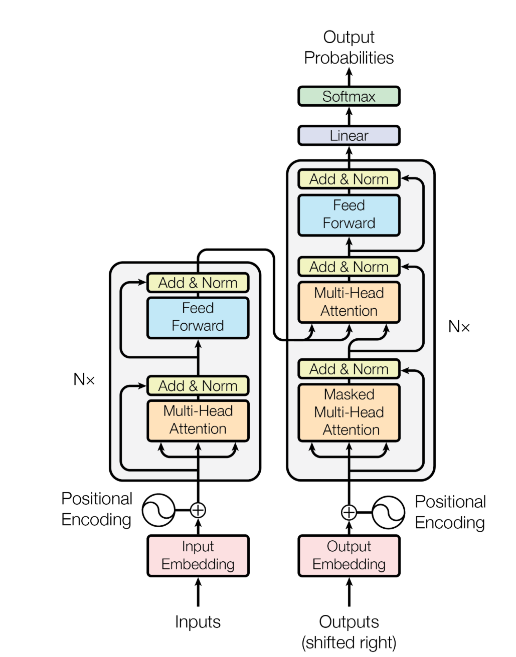
The figure shows the Transformer Block structure, with the right side displaying the decoder block and encoder block. Stacking N of these decoder and encoder blocks forms the Transformer.

4.1.1 Positional Encoding — Sinusoidal Encoding

$$P{E}_{(pos,2i)}=\sin \left(\frac{pos}{{10000}^{2i/d_{\text{model}}}}\right),P{E}_{(pos,2i+1)}=\cos \left(\frac{pos}{{10000}^{2i/d_{\text{model}}}}\right)$$

Variables: $pos$ — token position in sequence (0, 1, 2, ..., N-1); $i$ — dimension index; $d_{model}$ — model embedding dimension (512 in the paper); $10000$ — base frequency (configurable). The encoding is directly added to word embeddings: $X=Token+PE(pos)$.

Sinusoidal position encoding is the key design for introducing positional information into the Transformer. Since the Transformer's core is self-attention, which inherently lacks perception of input order — if word vectors were directly input, "我爱你" and "你爱我" would be treated as the same set. To solve this, positional information must be explicitly added to the input. Sinusoidal encoding requires no training; it generates position representations through fixed formulas, with the core idea of using sine and cosine functions at different frequencies to produce a unique encoding vector for each position that is also capable of perceiving relative position relationships.

Specifically, for the $pos$-th position and the $i$-th dimension of the encoding vector: even dimensions use sine, odd dimensions use cosine. The term ${10000}^{2i/d_{model}}$ determines the wavelength at different dimensions, forming a multi-scale encoding system: low dimensions (small $i$) correspond to high frequencies, enabling fine-grained distinction of adjacent positions; high dimensions (large $i$) correspond to low frequencies, capable of covering longer-distance relative relationships. Ultimately, each position receives an encoding vector of the same dimension as the word vector; the two are added as model input.

This design brings several significant advantages. First, it is completely deterministic and requires no extra parameters, avoiding increased model complexity or overfitting of trainable position embeddings. Second, through trigonometric function periodicity, encoding values are constrained to $[-1,1]$, numerically stable and easy to add to word vectors. More importantly, it naturally supports relative position modeling: for any fixed offset $k$, the encoding vector at $pos+k$ can be expressed as a linear transformation of the encoding vector at $pos$ (dependent only on $k$), enabling the self-attention mechanism to more easily learn relative position relationships between sequence elements, not just absolute positions. This property is particularly crucial for handling variable-length sequences and capturing local dependencies.

Q: Why is positional encoding needed?A: Since the Transformer has no recurrent or convolutional structure, the model itself is permutation-invariant. Positional encoding, added to token embeddings, provides the model with necessary sequential information.

Q: How does sinusoidal encoding provide positional information?A: For different positions pos, each dimension of the encoding vector takes different values, forming a unique pattern; the model learns this pattern to distinguish near and far positions.

4.1.2 Multi-Head Attention

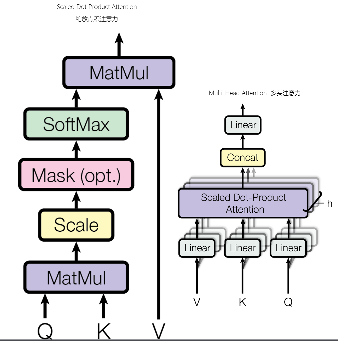
The attention mechanism mimics human attention — when viewing an image, we don't distribute attention evenly across every corner but selectively observe prominent parts. Similarly, the attention mechanism focuses on important parts of the input, expressed as larger weights. Attention is essentially weighted summation.

Multi-head attention is the Transformer's core innovation. By executing multiple attention "heads" in parallel, it enables the model to simultaneously attend to multiple dependency relationships from different perspectives and semantic levels, greatly enhancing complex pattern modeling capability.

1. Single-Head Attention and Its Limitations

Single-head attention computation is based on scaled dot-product attention. For input sequence $X$ (shape $[B,S,d_{model}]$), three weight matrices map it to query (Q), key (K), and value (V):

$$Q=X{W}^Q,K=X{W}^K,V=X{W}^V$$$$\text{Attention}(Q,K,V)=\text{softmax}\left(\frac{Q{K}^T}{\sqrt{d_k}}\right)V$$

Here $d_k=d_{model}$, and the scaling factor $\sqrt{d_k}$ prevents dot products from growing too large, pushing softmax into gradient saturation regions. Single-head attention's limitation is that it computes only one "query-key-value" relationship — like observing with only one pair of eyes — making it difficult to simultaneously capture syntactic structure, semantic associations, long-range dependencies, and other patterns.

2. Multi-Head Attention Design

Multi-head attention splits $d_{model}$-dimensional queries, keys, and values into $h$ independent heads, each computing attention in a lower-dimensional space ($d_k=d_{model}/h$), enabling the model to jointly extract information from multiple representation subspaces. Each head has its own projection matrices, allowing focus on different feature types — some heads may focus on local syntactic structure while others capture long-distance semantic dependencies.

3. Multi-Head Computation Process

Step 1: Multi-head splitting. Reshape and transpose Q, K, V from $[B,S,d_{model}]$ to $[B,h,S,d_k]$.

Step 2: Parallel head computation. For each head independently: ${\text{Head}}_i=\text{softmax}(Q_i{K}_i^T/\sqrt{d_k})V_i$

Step 3: Concatenation and final projection. $\text{Output}=\text{Concat}({\text{Head}}_1,...,{\text{Head}}_h)W^O$, restoring to $[B,S,d_{model}]$.

Original paper parameters: $d_{model}=512$, $h=8$, $d_k=d_v=64$, scaling factor $\sqrt{d_k}=8$.

Q: Why multiple heads instead of single?A: Parallel attention to different patterns; each head in a low-dimensional subspace ($d_k=64$) is more efficient than single head in high-dimensional space. Multi-head concatenation approximates high-rank matrix decomposition with stronger expressive power. Computation is also more efficient — heads compute in parallel, suitable for GPU acceleration, with total computation comparable to single head.

Q: Why divide by $\sqrt{d_k}$?A: Original hypothesis: when $d_k$ is large, dot product magnitudes grow large, pushing softmax into extremely low-gradient regions. Modern understanding: $\text{Var}(Q\cdot K)=d_k\cdot \text{Var}(q_i{k}_i)$, so dividing by $\sqrt{d_k}$ keeps variance stable. Benefits: maintains variance stability regardless of $d_k$, avoids gradient vanishing, stabilizes training.

4.1.3 LayerNorm and Residual Connections

1. What is Normalization?

Normalization scales data by specific rules into a uniform standard range or distribution. In probability theory: $x_{norm}=(x-\mu )/\sigma$. The process resets the data distribution to a standard state.

Original Transformer LayerNorm:

$$\text{LayerNorm}(v)=\gamma \frac{v-\mu }{\sigma }+\beta$$

Step by step: compute mean $\mu$ across features → compute std $\sigma$ → normalize → apply learnable $\gamma$ (scale) and $\beta$ (shift).

2. What is a Residual Connection?

The residual connection (skip connection) is a "shortcut" between network layers, allowing information to bypass certain layers directly:

$$\text{Output}=\text{Input}+\text{Layer}(\text{Input})$$

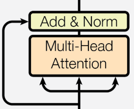
From an abstract perspective, this introduces shallow information flow — preventing information loss and error amplification as depth increases. Mathematically: the network learns the "residual" $F(x)=H(x)-x$ rather than directly learning the ideal mapping $H(x)$. If a layer doesn't need transformation, the network just learns $F(x)\approx 0$, preserving the input $x$.

3. LayerNorm + Residual Connection Collaboration

In the original Transformer, Post-Norm is used: $\text{output}=\text{LayerNorm}(x+\text{Sublayer}(x))$. This is: sublayer → residual → normalization.

Residual connections ensure gradients flow directly back, at minimum preserving identity mapping capability. LayerNorm standardizes the summed distribution, preventing numerical explosion/vanishing. Together they make 12-layer or even deeper networks trainable.

Q: Role of LayerNorm?A: Solves distribution shift and gradient instability problems; standardizes distribution; accelerates convergence; prevents vanishing/exploding gradients.

Q: Role of residual connections?A: Ensures direct gradient back-propagation; at minimum preserves identity mapping; provides stable information pathway; solves distribution instability in deep networks.

4.1.4 Feed-Forward Network and Activation Functions

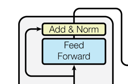
The original Transformer uses ReLU activation in the position-wise FFN:

$$\text{FFN}(x)=max(0,x{W}_1+b_1)W_2+b_2$$

Configuration: input/output dim = $d_{model}=512$, inner dim = $d_{ff}=2048$ (4× expansion). ReLU is applied only in the first layer. Why ReLU? Computationally efficient — derivative is simply 0 or 1, much simpler than Sigmoid/Tanh.

Q: What basic qualities must a good activation function have?A: 1. Nonlinear — otherwise deep networks collapse to single-layer linear models. 2. Differentiable — must support gradient descent and backpropagation (ReLU uses subgradient at x=0). 3. Computationally simple — called billions of times during training and inference.

---

4.2 Modern Transformer Variants

Since 2017, numerous high-quality papers have emerged — CommandA, OLMo, SmolLM, Gemma3, Qwen2.5, InternLM — with about 19 dense models released last year, most involving subtle architectural adjustments. Just learning the original standard architecture is insufficient to face the market's accelerating innovation.

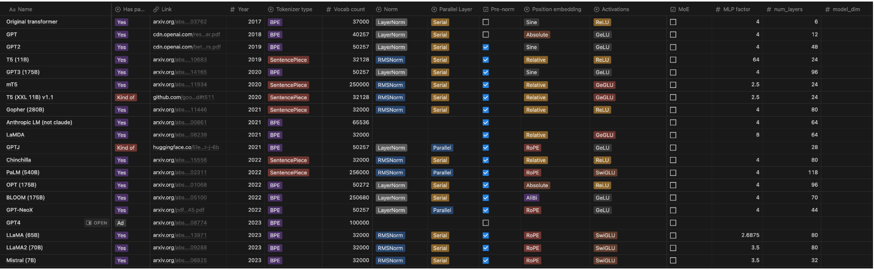
Looking at the architecture comparison table from the 2017 original to 2025's latest models, each module has seen innovation — position encoding has tried absolute, relative, RoPE, and even ALiBi. Around 2023, the field converged: almost everyone adopted RoPE due to superior performance. Llama-like architecture convergence trend — the Llama family, as the most popular open-source model (though this status is being challenged by Qwen), has reference significance for improved architectures.

We'll focus on activation functions, FFN, attention variants, and position encoding. After determining the architecture, we must select hyperparameters: hidden dimension size, MLP inner projection ratio, head count, vocabulary size — all critical decisions for actual LLM training.

4.2.1 Normalization

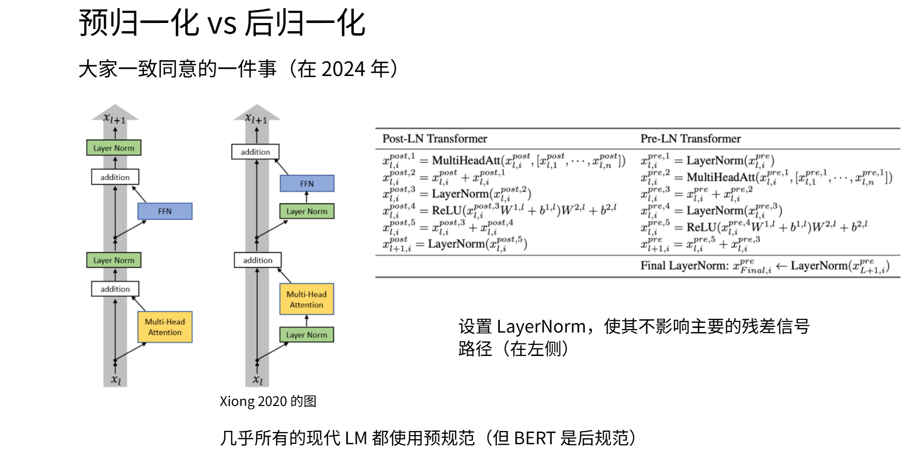
1. Post-Norm (original design)

$$X=\text{LayerNorm}(X+\text{Sublayer}(X))$$

This is the original Transformer design: residual stream passes through the sublayer, then added to input, finally LayerNorm.

2. Pre-Norm (modern mainstream)

$$X=X+\text{Sublayer}(\text{LayerNorm}(X))$$

Advantages: more stable training, no need for complex learning rate warmup, suitable for extremely deep networks (100+ layers). Now the default configuration for GPT-3, PaLM, and other large models.

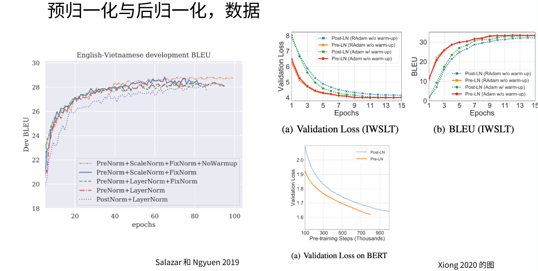
With Pre-Norm and other stabilization techniques, even without warmup, system performance matches or exceeds carefully-warmup-tuned Post-Norm LayerNorm. Various explanations exist — avoiding inter-layer gradient decay, maintaining constant gradient scale — but the most modern understanding is simply that Pre-Norm is inherently a more stable training architecture.

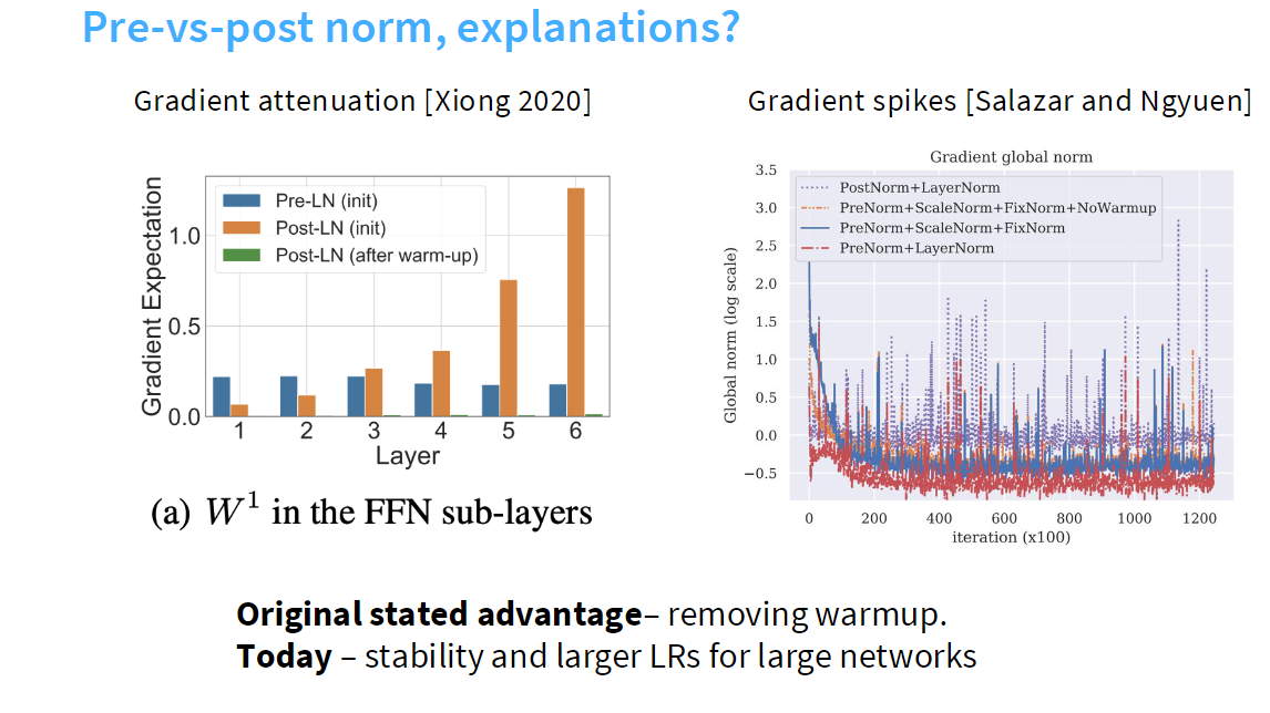
The core design philosophy is "keep your residual stream clean." In Pre-Norm, input $X$ flows unimpeded from bottom to top of the model through residual connections, forming an obstacle-free gradient highway. Backpropagation gradients flow losslessly without attenuation or explosion from repeated LayerNorm scaling on the residual path. Post-Norm, with each Transformer block applying normalization, causes complex gradient norm fluctuations during backpropagation.

Today, Pre-Norm and other LayerNorm techniques are widely used as stability aids when training large neural networks.

3. "Double Normalization"

Why must LayerNorm only be placed before sublayers? It can also be placed after. Recent research even places LayerNorm both before and after modules. Grok and Gemma2 adopt this approach; OLMo2 only places LayerNorm after FFN and multi-head attention. Evaluations suggest this new approach is more stable and performs better when training larger models.

4. Simplified Variant: RMSNorm (Most Popular)

LayerNorm's mean and std computation is expensive and not strictly necessary for Transformers. Essentially all models have switched to RMSNorm, whose core change is: directly removing the mean-centering step (and the bias term). LLaMA, PaLM, Chinchilla, T5 have all adopted RMSNorm. Performance is comparable to LayerNorm, but RMSNorm is faster — no mean subtraction means fewer operations; no bias term $\beta$ means fewer parameters to load from memory to compute units.

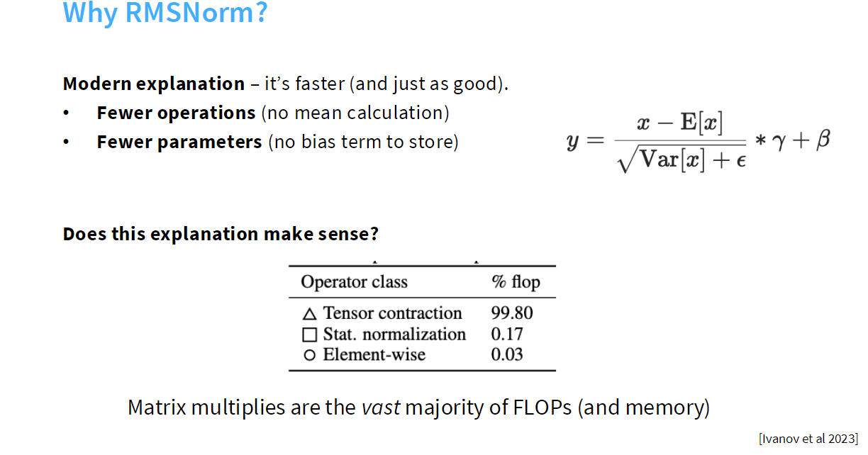
LayerNorm has stronger expressive power, but RMSNorm has almost no performance loss in practice with significant speed advantages. This involves system-architecture co-design: improving arithmetic intensity — prioritizing high-density computations like matrix multiplications, avoiding GPU idling from moving fragmented memory data. Mean subtraction contributes limited expressive power, so removing it is reasonable.

Although mean subtraction's FLOPs are only ~0.17% of total, runtime does not equal FLOP count. Statistical normalization involves substantial memory movement, and memory access is far slower than computation. Depending on workload, such operations can consume up to 25% of runtime (higher proportion on smaller models). RMSNorm effectively reduces the burden of extremely low arithmetic intensity operations, delivering significant speedup.

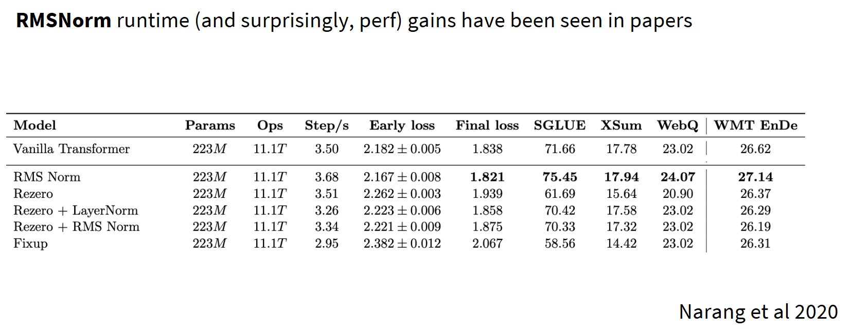
In small Transformer experiments switching to RMSNorm, training steps per second clearly increase, sometimes even improving model performance. This is a "free lunch" system-level optimization, now widely adopted.

RMSNorm formula (removing mean normalization, retaining only variance normalization):

$$\text{RMSNorm}(v)=\gamma \frac{v}{\sqrt{\frac{1}{d}\sum _{i=1}^d{v}_i^2+\epsilon }}$$

Narang et al. (2020) ablation experiments clearly show: baseline Transformer processes 3.5 steps/second while RMSNorm reaches 3.68 steps/second, with final loss also lower than baseline.

Q: Why is LayerNorm in the residual (Post-Norm) bad?A: Intuitively, residual connections maintain identity mapping from top to bottom layers, greatly benefiting gradient propagation in extremely deep networks. LSTM-like state space models struggle with gradient backpropagation, while residual connections completely avoid this. Inserting LayerNorm in the middle may interfere with this gradient behavior. Now many models have shifted to RMSNorm — this has become a consensus improvement.

5. Normalization New Trend: Double Normalization

In recent years, a more aggressive normalization strategy has emerged: placing LayerNorm both before and after sublayers. Typical examples include Grok and Gemma 2; OLMo 2 additionally places LayerNorm after attention and FFN.

The design intuition stems from practical experience: "If you encounter stability issues, sprinkling some LayerNorm everywhere often solves the problem." Though lacking theoretical elegance, this strategy has been repeatedly validated to significantly improve deep Transformer training stability with almost no performance degradation.

The design philosophy is "keep your residual stream clean." Whether Pre-Norm or double normalization, the core idea is maintaining an obstacle-free gradient highway. In Grok-2, each of its 64 Transformer blocks contains pre_attn_norm, post_attn_norm, pre_moe_norm, post_moe_norm — four normalization layers. Gemma 2 uses RMSNorm both before and after attention and FFN sublayers.

4.2.2 Feed-Forward Network

Original FFN: $\text{FFN}(x)=max(0,x{W}_1+b_1)W_2+b_2$ — two linear layers with bias + ReLU.

Modern implementations (non-gated variants) have removed all bias terms (b). Matrix multiplication alone is sufficient for model operation; another reason is optimization stability. While nobody fully understands why bias terms are particularly detrimental to stability, clear empirical observations show that removing bias terms generally stabilizes large neural network training. Many implementations now completely omit bias terms, training purely in matrix-multiplication settings.

Removing bias terms from linear and normalization layers is not only for reduced memory overhead and improved arithmetic intensity — there's also a widely observed but not fully theoretically explained phenomenon: bias terms may induce training instability. Despite the exact mechanism remaining an open question, extensive empirical evidence shows removing bias typically reduces gradient spikes and numerical divergence risks. "Bias-free" design has thus elevated from simple system optimization to a default stability safeguard.

Modern non-gated FFN: $\text{FFN}(x)=max(0,x{W}_1)W_2$. The rationale for removing bias is almost identical to RMSNorm's.

4.2.3 Activation Functions

Since the invention of Transformer/deep learning, improving activation functions has been a hot area — ReLU, GeLU, Swish, ELU, GeGLU, ReGLU, SeLU, SwiGLU, LiGLU.

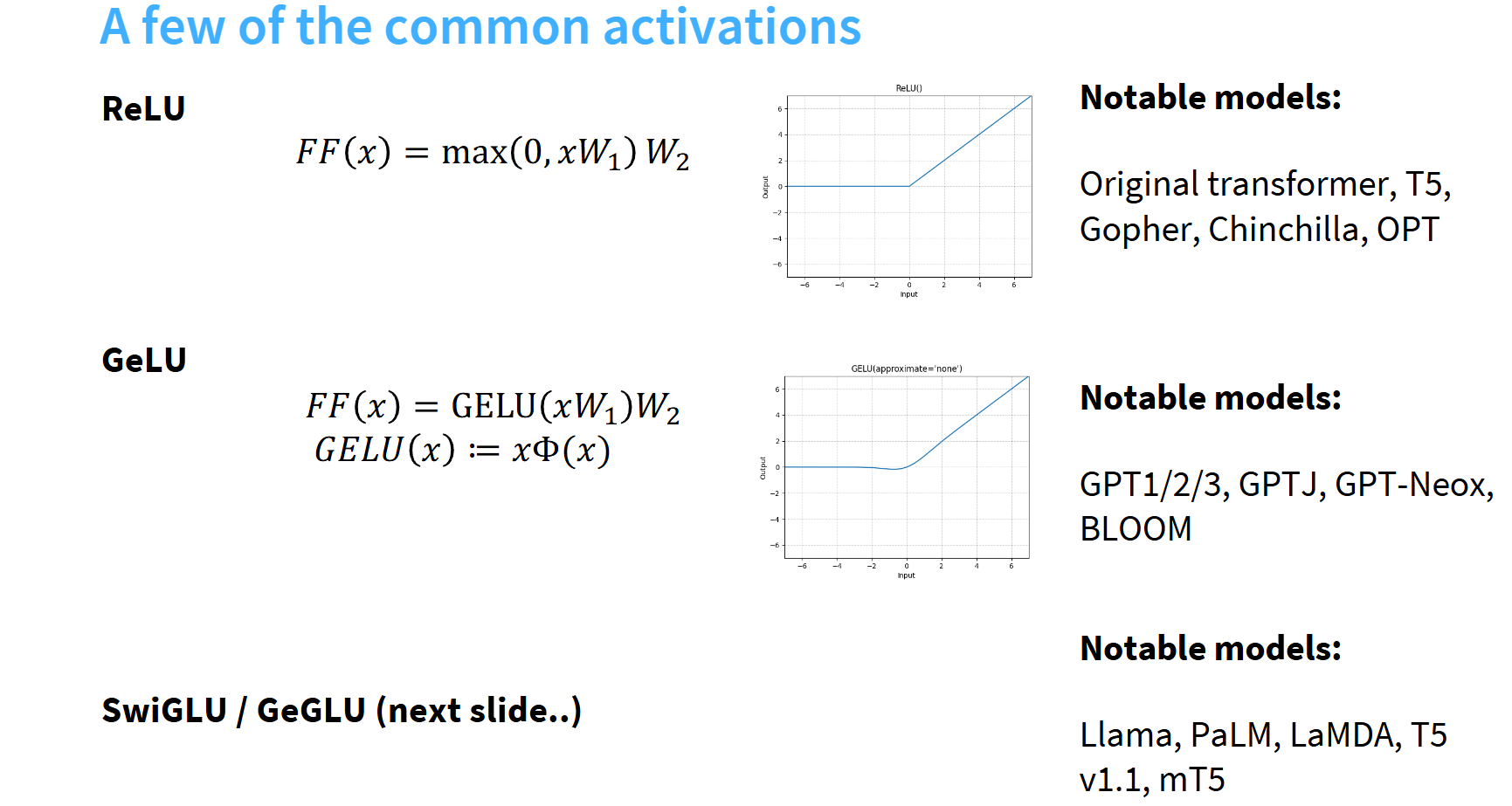
1. ReLU: $max(0,x)$. The most basic activation function, extremely simple. Advantage: simple derivative.

2. GeLU (Gaussian Error Linear Unit): $\text{GeLU}(x)=x\cdot \mathrm{\Phi }(x)$ where $\mathrm{\Phi }(x)$ is the standard Gaussian CDF. Essentially like ReLU but with a bump at the origin — smoother, more differentiable than ReLU. Used by GPT-1/2/3 and GPT-J. Disadvantage: more computationally complex than ReLU. In practice, polynomial approximations are used due to expensive exact error function computation.

3. Gated Linear Unit (GLU) Family:

GLU inspired the GLU family. Essentially all post-2023 models use gated linear units.

GLU (family ancestor): $\text{GLU}(x)=(xW)\odot \sigma (xV)$

GLU can be understood as a "gating + content" dual-channel mechanism:

1. Content channel: $xW$ provides original information
2. Gating channel: $\sigma (xV)$ generates 0-1 "switches," determining each neuron's throughput
3. Dynamic activation: Each token gets different gating values, achieving input-dependent sparsity

Like smart blinds — dynamically adjusting each slat's opening based on input, rather than traditional activation's "fully open/fully closed" binary behavior.

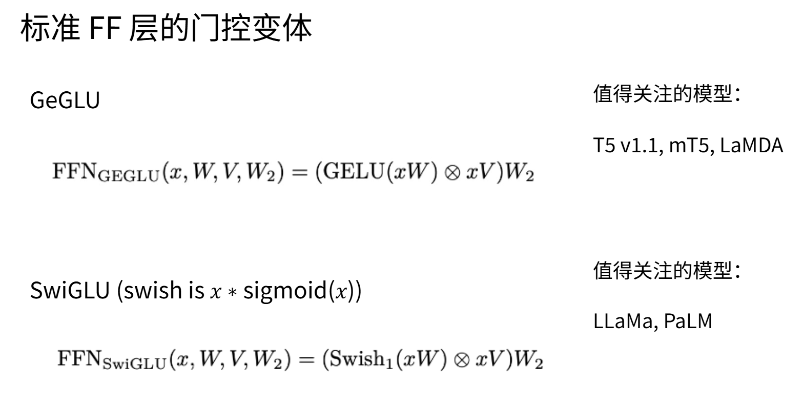
GeGLU (Gated GELU): $\text{GeGLU}(x)=\text{GELU}(xW)\cdot (xV)$. Improvement: smooth GELU replaces Sigmoid as gating function. Advantage: more stable gradients, slightly better performance. Used by Google models (T5, Gemma2/3).

SwiGLU (Swish GLU): $\text{SwiGLU}(x)=\text{Swish}(xW)\odot (xV)$ where $\text{Swish}(x)=x\cdot \sigma (\beta x)$, typically $\beta =1$. Advantage: further performance improvement over GeGLU. Cost: highest computational cost. SwiGLU is basically what most current models use — LLaMA series, PaLM, OLMo, etc.

Parallel vs. Serial Blocks

Standard Transformer blocks are serial: attention first, then FFN. Around 2020, GPT-J and PaLM experimented with parallelized block design — adding attention and FFN outputs together directly into the residual stream, aiming to reduce latency through operator fusion. However, this parallel structure has been essentially abandoned in the past two years. The main reason: parallelization effectively halves model depth, severely weakening expressive power. With hardware and software optimization advances, serial computation is sufficiently efficient; parallel marginal benefits can no longer compensate for performance loss. Post-2024 models (LLaMA 3, Qwen 2.5) all return to serial design.

Q: Are gated units effective?A:

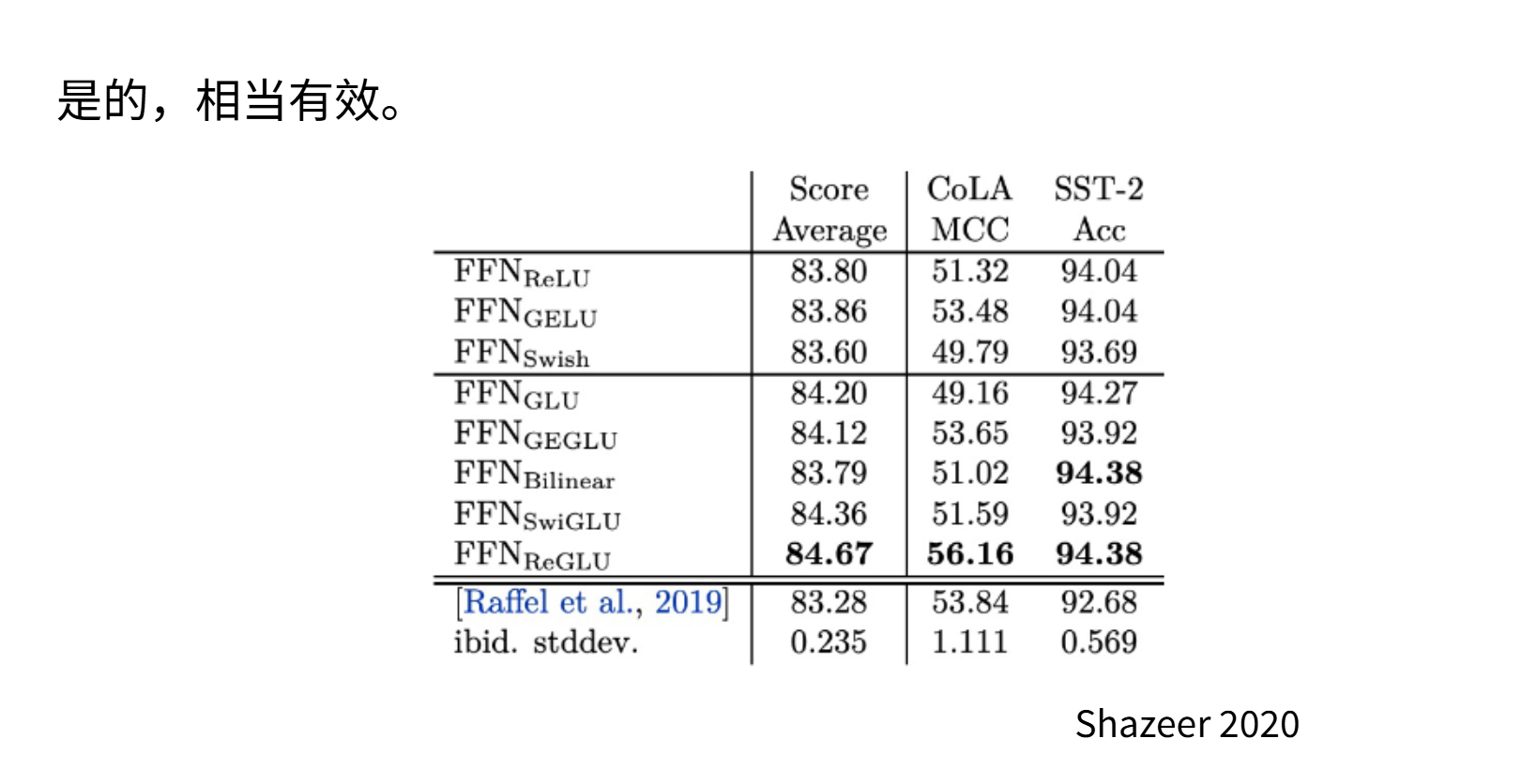
Noam Shazeer's original paper evaluated all GLU variants. These data are relatively early, but you can see performance on CoLA and SST-2 tasks. GLU variants consistently outperform: GLU achieves 84.20, 84.12, 84.36, 84.67 respectively. Notably, this is 2020 research, and they even provided standard deviations to assess result significance — these results are indeed statistically significant. This is good empirical evidence.

Narang et al.'s 2020 paper is also worth noting. This high-quality study tested various architectural variants on T5-like models. Again, gated linear unit variants consistently achieve lower loss values, with bolded rows corresponding to GLU variants. This advantage pattern has persisted to this day.

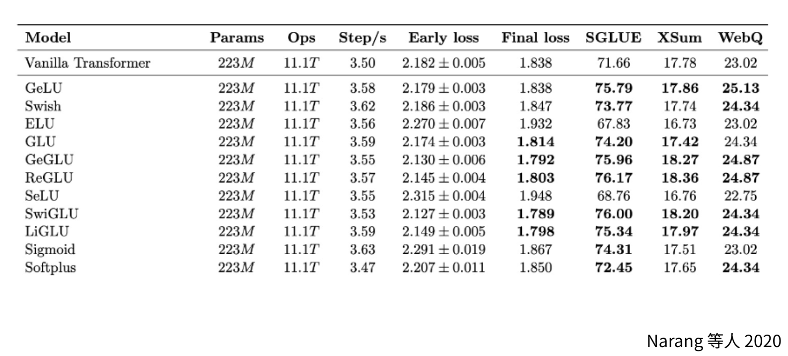
Regarding gating and activation functions, different models have many variants, but gated linear units have essentially become the mainstream choice. However, it must be clear that excellent models don't necessarily require GLU. We cannot consider it indispensable just because of its slight advantage and widespread use. There are indeed many high-performance model cases that don't use GLU. For example, GPT-3; the newer Nemotron 340B used squared ReLU — a design not seen before. And Falcon 211B uses ReLU activation. Both are relatively high-performance models. Therefore, this is clearly not a necessary choice. Existing evidence does suggest that SwiGLU and GeGLU bring consistent performance gains.

4.2.4 Position Encoding

Discussing position encoding evolution fully would take forever. We'll focus on RoPE — the position encoding used by almost all advanced models — with only brief mentions of others.

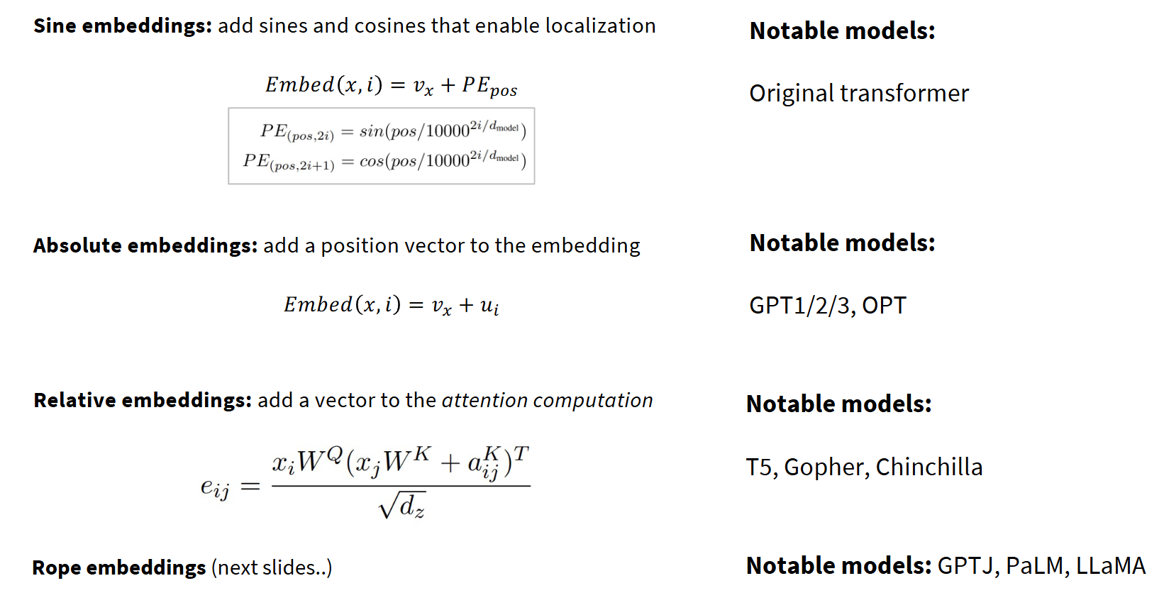
1. Absolute Embedding — Sinusoidal Embedding

Assigns a unique encoding vector to each sequence position, added to word embeddings: $\text{Final Embedding}=\text{Token Embedding}+\text{Positional Embedding}$. T5 and others use relative position encoding. Sinusoidal encoding is a type of absolute position encoding — the original Transformer's parameter-free method using sine/cosine functions to generate unique patterns. Advantages: parameter-free, computationally efficient, theoretically extensible to unseen longer sequences. Disadvantages: absolute position perception cannot directly model relative distance; long sequence performance degrades.

2. Relative Embedding — RoPE (Rotary Position Embedding)

Core idea: model relative distance between tokens rather than absolute positions. Instead of encoding absolute positions, explicitly introduce relative position information into attention computation by adding vectors that make the model attend to inter-token distance. RoPE is a type of relative embedding.

RoPE was first proposed by Jianlin Su in 2021 in "RoFormer: Enhanced Transformer with Rotary Position Embedding." GPT-J was among the first notable open-source models to adopt RoPE. Today, RoPE has multiple context-length extension algorithms — a critical component of modern production-grade language models. Even in small-scale, short-context scenarios, empirical effects are very significant; RoPE has essentially won the position embedding competition.

What is rotation? The concept relates to complex numbers. In 2D space, a vector $v=(x,y)$ represented as complex number $z=x+iy$; rotating by $\theta$ is equivalent to multiplying by $e^{i\theta }$, which in vector space equals multiplying by a rotation matrix:

$$R(\theta )=\left[\begin{array}{cc}\cos \theta & -\sin \theta \\ \sin \theta & \cos \theta \end{array}\right],R(\theta )\cdot v=\text{rotated vector}$$

Rotation matrix properties: orthogonal (inverse = transpose), determinant = 1 (preserves vector length), periodic ($R(\theta +2\pi )=R(\theta )$), additive ($R(a+b)=R(a)R(b)$ — we'll use this right away).

When we rotate both Q and K matrices: $Q_1=R(m)Q$, $K_1=R(n)K$. During attention computation:

$$Q_1\cdot K_1^T=R(m)R(n{)}^{T}Q{K}^T=R(m)R(-n)Q{K}^T=R(m-n)Q{K}^T$$

We achieve relative position information: the inner product depends only on the relative distance $(m-n)$!

For high dimensions, RoPE splits the vector into multiple 2D sub-blocks, independently rotating each at different frequencies ${\theta }_i={10000}^{-2i/d}$. Some dimensions rotate quickly (capturing high-frequency, short-range information) while others rotate slowly (capturing low-frequency, long-range positional information).

Unlike the original paper's sinusoidal embedding, RoPE operates within the attention layer itself — each attention computation intervenes at that layer to obtain positional information.

Why everyone loves RoPE: 1. Explicit relative position — inner product depends only on relative distance, aligning with attention's essence. 2. Unlimited extrapolation — orthogonal rotation extends infinitely. 3. Parameter-free and efficient — zero extra parameters, negligible compute overhead.

P-RoPE (Proportional RoPE) — Gemma 4, 2026

A lightweight RoPE variant: only rotates the first 25% of dimensions per attention head, keeping the rest unchanged. The hypothesis: high-frequency position changes can be sufficiently expressed through a minority of dimensions, while most dimensions remain pure content representations, reducing position signal interference in semantic space. Gemma 4 even uses a "dual RoPE" configuration: sliding window layers use standard RoPE (theta=10,000) while global attention layers use P-RoPE (theta=1,000,000).

4.2.5 Attention Variants

In traditional attention, each head gets its own unique Q, K, V matrices — for $h_1$, $Q_1,K_1,V_1$ are three different matrices; $h_2$ gets different $Q_2,K_2,V_2$.

1. KV Cache

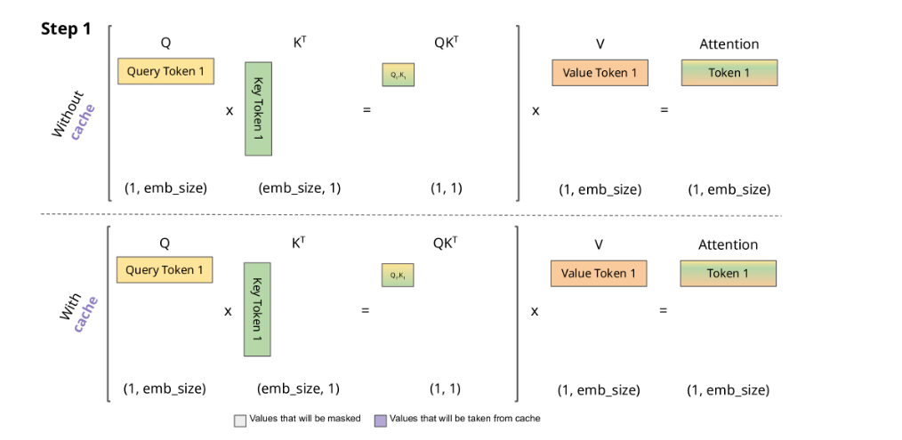
During autoregressive generation, we generate one token at a time. We store historically computed K and V values — this avoids recomputing them for each new token. This is called the KV cache. (Detailed in the inference chapter.)

2. MQA (Multi-Query Attention) and GQA (Grouped-Query Attention)

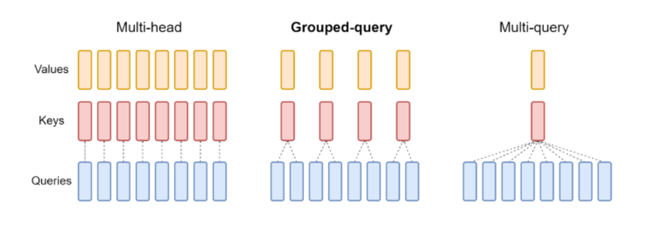
To reduce KV Cache memory pressure, two variants emerged:

• MQA: All heads share a single K and V. Dramatically reduces cache size (by factor of $h$). Slight quality trade-off.
• GQA: Groups of heads share K and V. Balances quality and efficiency. Used by LLaMA 2/3, Gemma, etc. — the current mainstream compromise.

Why Is GQA So Effective? From the Perspective of KV Cache Arithmetic Intensity

GQA not only saves memory — more critically, it addresses the Arithmetic Intensity bottleneck in the autoregressive inference phase.

During autoregressive generation, every step requires reading all historical Keys and Values from the KV Cache for incremental computation. At this point, memory access surges while compute stays constant, causing arithmetic intensity to plummet — the GPU spends most of its time waiting for data movement. Its arithmetic intensity is roughly proportional to:

$$\frac{1}{N/D+1/B}$$

where $N$ is sequence length and $D$ is model dimension. The $N/D$ term is the culprit behind the drastic efficiency degradation for small models or long sequences.

MQA/GQA's core contribution: by having multiple query heads share the same Key/Value set, the $N/D$ term in the arithmetic intensity denominator gets multiplied by the number of heads $H$, becoming $N/(H\cdot D)$. This is equivalent to using more query heads to "amortize" the cost of memory access, dramatically improving throughput at the hardware level — far beyond simply "saving memory." This is why GQA can achieve near-MQA inference efficiency with almost no performance loss.

4. Sparse / Sliding Window Attention

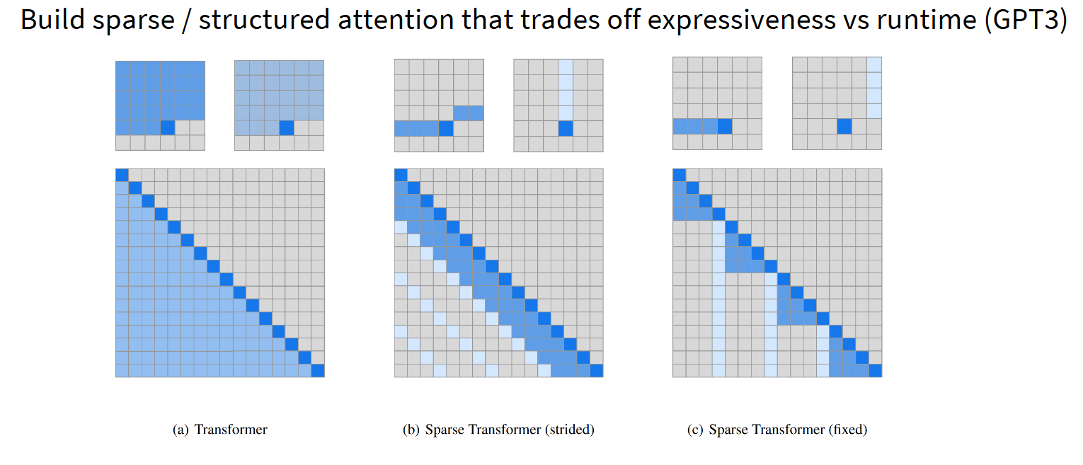
Looking back to 2019, OpenAI published an excellent paper exploring how to build models with longer attention spans. Their proposed solution was to design sparse attention patterns — not attending to the entire sequence, but focusing on local windows within each block, supplemented by diagonal attention patterns to pass information across blocks. Through such sparse or structured attention, one can balance expressiveness and runtime efficiency.

GPT-3 adopted such techniques at its initial release to achieve larger attention windows. Sliding window attention is another variant of this idea — at each layer, only attending to the neighborhood of the current position. This effectively controls the total resources needed for processing long texts, with the effective receptive field equal to local range × number of layers. While these are earlier ideas, modern implementations have evolved significantly.

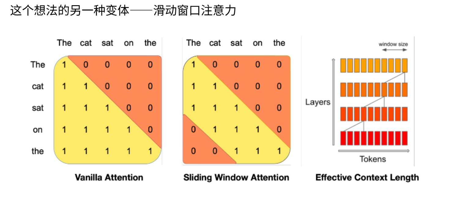
Recently, papers from LLaMA 4, Gemma, and Cohere Command A proposed an ingenious scheme: construct groups of four Transformer blocks, where the bottom block uses full self-attention but without any position embeddings (neither RoPE nor other position encodings) — completely lacking position awareness yet achieving complete self-attention functionality. And this only happens once every four blocks. The three blocks above it use sliding window attention with RoPE. This is actually a very clever trick — it controls system-level factors since full attention only occurs occasionally, while also handling length extrapolation since RoPE only processes local context windows. For truly long-range dependencies, no position embedding is needed at all, enabling very aggressive extrapolation.

5. Modern Sliding Window Attention Hybrid Paradigm

Early sliding window attention was typically used as a cheap substitute for global attention. But between 2024–2025, a global + local alternating hybrid paradigm rapidly became mainstream:

Cohere Command A pioneered an alternating pattern with groups of 4 Transformer blocks: 1 layer uses full global attention (able to see all historical tokens), while the remaining 3 layers use sliding window attention (only attending to local context).

Cohere Command A's specific configuration is 3 sliding window layers (window 4,096) + 1 global attention layer. OLMo 2 uses global attention at the 4th layer of every 4-layer group and at the final layer. Qwen 3.5 alternates Gated DeltaNet (linear attention) with standard attention at roughly a 3:1 ratio — Gated DeltaNet combines Mamba2's gated decay mechanism with the Delta rule.

This design has been widely adopted by the latest models such as LLaMA 4, Gemma 4, OLMo 3, enabling ultra-long context at controllable computational cost. Further exploration comes from Qwen 3.5, which replaces sliding window layers with a state space model (Gated DeltaNet) while preserving the "global attention every few layers" alternating structure, thereby fusing linear attention with standard attention.

This paradigm cleverly exploits the hierarchical property of "local information converging upward into global information layer by layer," striking an excellent balance between inference efficiency and long-range dependency modeling.

6. MLA: DeepSeek's Multi-Head Latent Attention

MLA (Multi-head Latent Attention) is an innovative attention architecture introduced by DeepSeek, using low-rank joint compression to dramatically reduce KV cache requirements during inference while maintaining performance and significantly boosting efficiency.

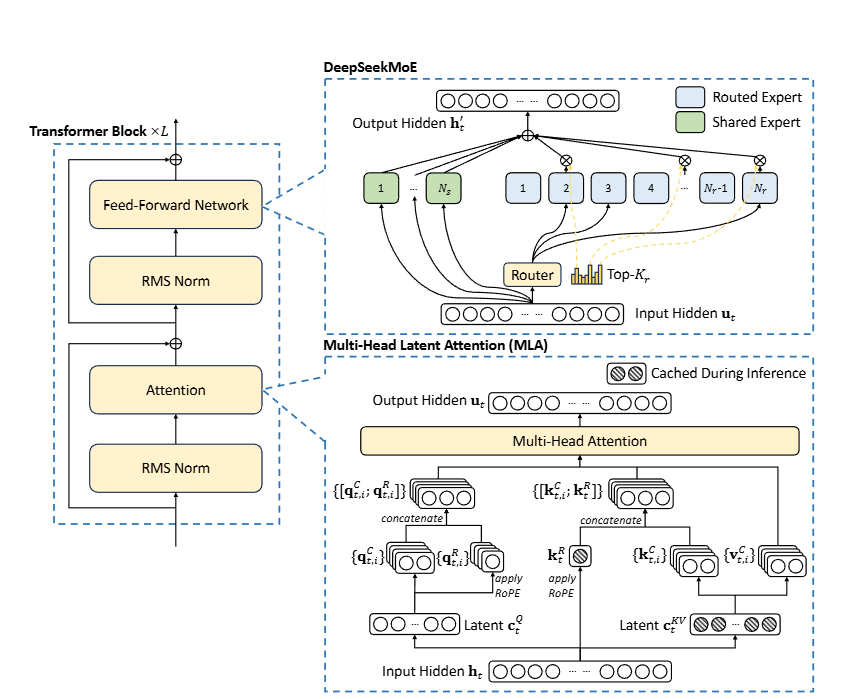
Reducing KV cache by 93% — the DeepSeek-V2 architecture diagram is shown above. MLA ensures efficient inference by dramatically reducing the KV cache needed for generation.

Traditional Transformer models typically use Multi-Head Attention (MHA), but during generation, the massive Key-Value (KV) cache becomes a bottleneck limiting inference efficiency. To reduce KV cache, Multi-Query Attention (MQA) and Grouped-Query Attention (GQA) were proposed. They require smaller KV caches, but their performance never matches MHA.

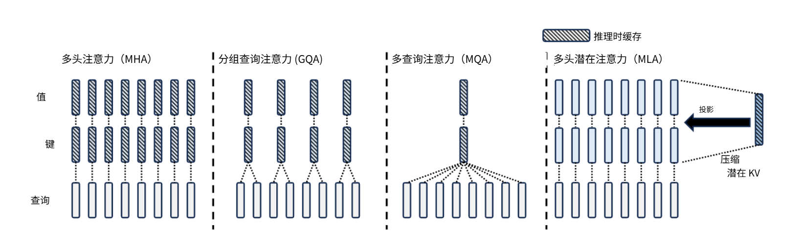
Traditional Transformers use MHA where each attention head independently caches Key and Value vectors. For a model with $L$ layers, hidden dimension $d$, and $h$ heads, KV cache complexity is $O(L\cdot h\cdot d)$ — the main bottleneck for long-sequence inference.

MLA's core breakthrough is jointly compressing the Keys and Values of all attention heads into a shared low-dimensional latent space, rather than compressing each head individually. The specific implementation is:

$$K^{\prime }=K\cdot W_K^{down},V^{\prime }=V\cdot W_V^{down}$$

where $W_K^{down}$ and $W_V^{down}$ are down-projection matrices mapping the original high-dimensional KV to a latent space of dimension $r$ (typically $r\ll d$). During inference, only the compressed latent vectors need to be cached, reducing cache complexity to $O(L\cdot r)$.

MLA's main steps:

Input mapped to latent space: Given input (where n is sequence length, d is feature dimension), project it into latent space via mapping function f. This dramatically reduces memory footprint when storing KV.

$$c_K=x\cdot W_K^{down}\in {\mathbb{R}}^{L\times r}$$$$c_V=x\cdot W_V^{down}\in {\mathbb{R}}^{L\times r}$$

Before attention computation, up-project the cached compressed KV back to the original space:

$$K=c_K\cdot W_K^{up}\in {\mathbb{R}}^{L\times (h\cdot d_h)}$$$$V=c_V\cdot W_V^{up}\in {\mathbb{R}}^{L\times (h\cdot d_h)}$$

Some might argue: this reduces KV cache memory but clearly increases computation — every attention computation requires decompression, and after computation, recompression. Indeed, there's no perfect solution; we must weigh trade-offs. Clearly, memory is far more precious than time, and the added computation is within expectations. Compared to the memory saved, memory is clearly more important.

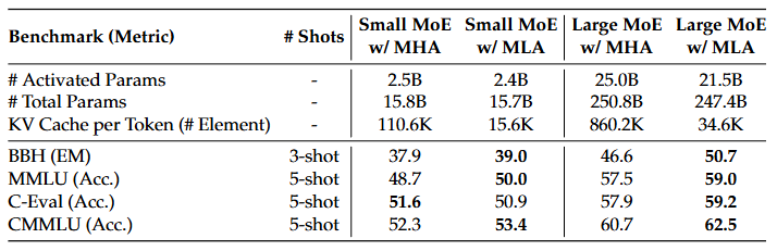
Comparison of MLA and MHA on difficult benchmarks. DeepSeek-V2 (using MLA) outperforms MHA while requiring significantly less KV cache. Although MLA is not widely used — only in the DeepSeek series — DeepSeek's outstanding model performance has already demonstrated this technology's capability.

7. DSA (DeepSeek Sparse Attention)

DeepSeek Sparse Attention (DSA) is a fine-grained dynamic sparse attention mechanism introduced in DeepSeek-V3.2-Exp, and the first technique named after DeepSeek. By intelligently filtering key information, it reduces long-context inference cost by 60–70% with almost no quality loss.

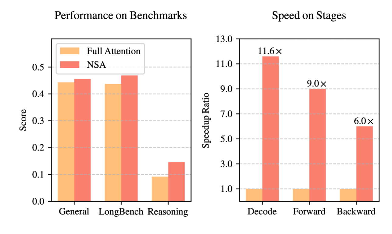
According to the paper published by DeepSeek (which won the ACL 2025 Best Paper award), NSA slightly outperforms full attention in scores while thoroughly dominating in speed. For 64k-length sequence processing, NSA achieves significant computational acceleration across all phases of full attention (decoding, forward propagation, and backward propagation).

Reviewing Previous Attention Mechanisms

Previous attention mechanisms all followed a fully-connected paradigm — each Query token must compute attention with all historical tokens. The problem is that for model inference, truly critical tokens are actually very few; most tokens are irrelevant. Just like in a sentence, not every character is key — there are many filler words and particles.

DSA Core Principle

DSA optimizes this scenario through "filter first, compute later" — scan historical tokens, compute importance scores, and only tokens with sufficiently high scores enter attention computation. The core architecture consists of two components: the Lightning Indexer and the Top-k Selector.

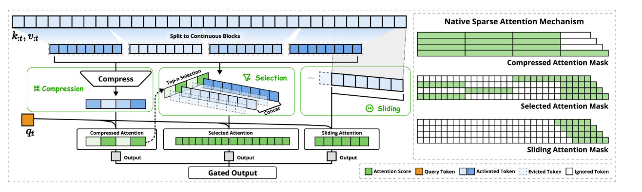
1. Lightning Indexer:

For each Query token, rapidly scans historical tokens and computes "importance proxy scores." It is a lightweight network using far fewer attention heads than the main model, running at FP8 low precision, quickly scanning all historical tokens and computing scores.

2. Fine-grained Top-k Selection

Based on index scores, dynamically constructs a dedicated Top-k set for each Query, with k typically = 2048, independent of sequence length L, forcibly reducing complexity to $O(L\cdot k)$, compared to traditional attention's $O(L^2)$.

Most impressively, DSA is a flexible plug-in — models not originally trained with DSA can adopt it through simple training.

8. CSA and HCA Mixed Attention Architecture in DeepSeek V4

CSA stands for Compressed Sparse Attention, and HCA stands for Heavily Compressed Attention.

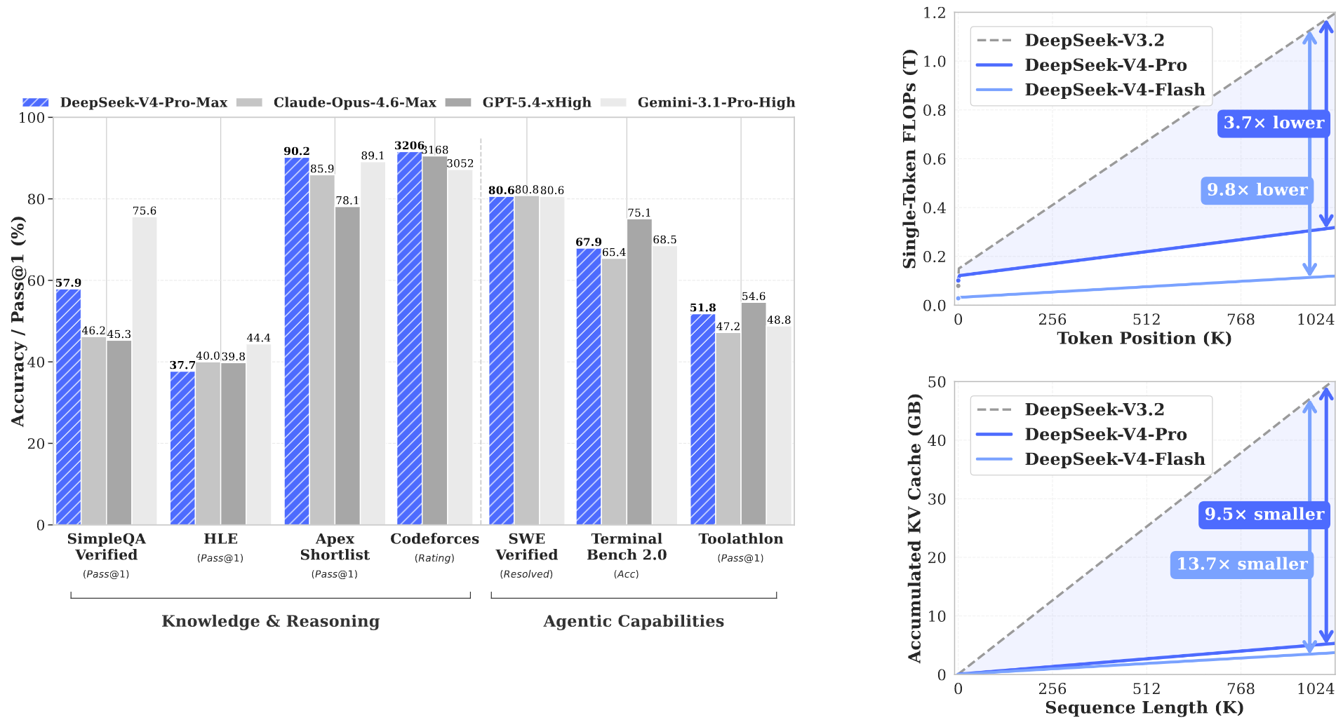
From the figure above, we can see that DeepSeek-V4-Pro's performance basically matches top-tier closed-source models, yet with ~1.6T parameters, DeepSeek V4 Pro's KV cache and per-token compute are far lower than DeepSeek V3.2. Part of this is the structural advantage of the MoE architecture itself, but a major improvement in V4 Pro is the optimization of the attention architecture. DeepSeek V4 utilizes a CSA and HCA hybrid alternating architecture to reduce KV Cache and computation.

The CSA and HCA hybrid attention architecture is based on MQA design. The core logic is using the alternating structure of CSA and HCA for division of labor — CSA preserves the ability to process fine-grained information, HCA achieves extremely low-cost global long-term memory, combined with sliding windows to capture the most immediate local information.

---

I. CSA: Balancing Compression and Sparsity

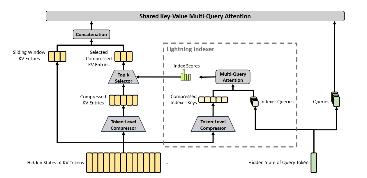
CSA's design philosophy is to dramatically reduce computation while preserving high-resolution attention to key details. It proceeds in two steps: compress first, then sparsely select.

1. KV Cache Compression

This avoids directly processing massive raw KV caches. It compresses the KV cache of every m tokens into one entry — a block-level representation.

Not simple average pooling, but through a learnable weighted compression mechanism. The model computes a compression weight for each token, then sums the KV pairs of these m tokens by weight, fusing them into one compressed entry. During compression, adjacent compressed blocks share some tokens. This smooths boundary information, preventing information fragmentation from hard partitioning. This reduces KV cache规模 to 1/m of the original. In V4, m is set to 4. A small set of sliding window KV entries is also introduced to enhance local fine-grained dependencies.

2. DSA Takes the Stage

After compression, if dense attention were computed over all blocks, complexity would still be quadratic. CSA then uses sparse attention to select only the most relevant blocks.

First, the Lightning Indexer rapidly computes relevance scores between the current query token and all compressed KV blocks. Based on index scores, only the top-k highest-scoring compressed KV blocks are retained for the current query token. Core attention computation drops from $O$(sequence length) to $O(k)$, decoupled from sequence length. In V4, k=512 for Flash, k=1024 for Pro.

CSA layer execution flow: first apply learnable weighted compression to KV cache, then use Lightning Indexer at low precision to select the most relevant Top-k blocks, and finally compute core attention only on the sparsely selected blocks.

---

II. HCA: Extreme Compression for Global Context

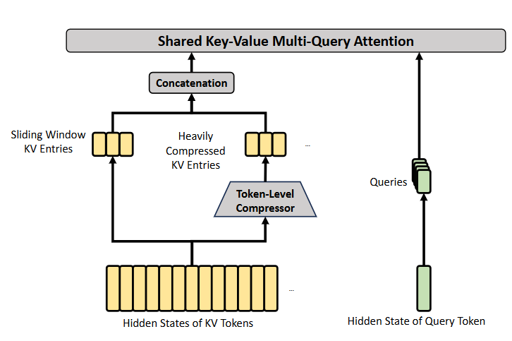
HCA's goal is to maintain a global contextual view covering hundreds of thousands of tokens at extremely low cost. It only does compression, no sparse selection.

HCA is similar to CSA, but the compression ratio m is much larger than CSA's — local information from many tokens is fused. Because compression is aggressive enough, sequence length becomes extremely short. So HCA can perform dense attention on this very short sequence, allowing every token to see the entire global context without loss. Since the sequence is short, computational cost is fully controllable.

---

4.3 Hyperparameter Considerations and Design Principles

When you're suddenly asked to train a new language model, you'll have many questions about hyperparameters, because there are quite a few. A key point you should realize: across different successful models, only a handful of hyperparameters are actually tuned. The field follows fairly clear empirical rules and guiding principles. For instance, how much should the feed-forward network size be expanded? How should the number of attention heads be set? What vocabulary size is appropriate? How much larger should the FFN size be than the hidden size? How many heads, and should num_heads always divide the hidden size evenly? How do people scale these models — deeper or wider?

This chapter will answer all these questions!

4.3.1 Feed-Forward Network

Let's start with a simple feed-forward layer. Assume this is the ReLU version with bias(b):

$$FFN(x)=max(0,x{W}_1+b_1)W_2+b_2$$

This involves two hyperparameters: $d_{model}$ (the dimension of input x, i.e., FFN input dimension) and $d_{ff}$ (feed-forward network dimension, i.e., FFN hidden layer output dimension), which ultimately projects back to $d_{model}$ dimension. When you plan to scale up the model, the FFN typically scales up too. The specific multiplier is actually a long-standing consensus in the field: nearly all researchers using ReLU-type MLPs set $d_{ff}$ to 4× $d_{model}$.

$$d_{ff}=4d_{model}$$

This is a validated convention, though it's not 100% universally correct — there are some exceptions:

Exception 1: GLU Variants Adjust the Expansion Factor to 2/3

Through simple calculation, for GLU variants, $d_{ff}$ should be set to $(8/3)d_{model}$.

$$d_{ff}=(8/3)d_{model}$$

Observing existing models, many follow this empirical rule — (8/3) ≈ 2.66.

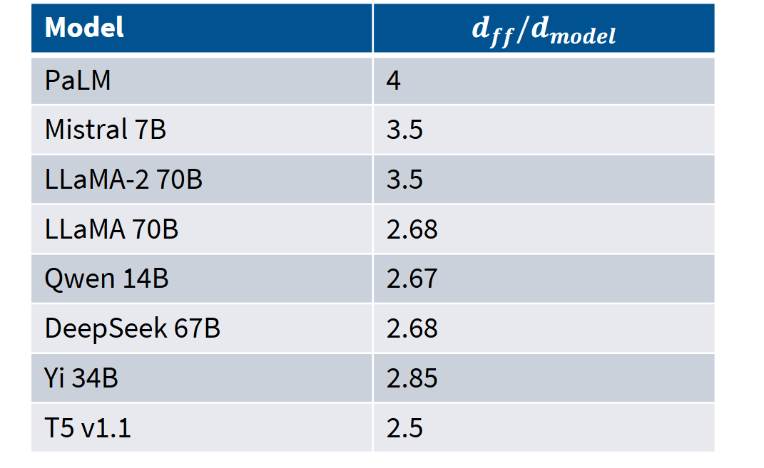
Taking PaLM as an example, Mistral and LLaMA's settings are slightly larger. Although they are all GLU models, they don't follow the 2.6× rule. But LLaMA-1, Qwen, DeepSeek, Yi, and T5 all roughly follow the ~2.6× setting.

Exception 2: T5 Model

To some extent, LLM training is like a hyperparameter replication game, causing the field to develop conservatively. But the T5 model demonstrated remarkable boldness — the Google team indeed made some quite daring attempts. In the 11B parameter T5 model, they adopted an astonishing configuration with hidden dimension set to just 1024. But their $d_{ff}$ (feed-forward network dimension) and its upward projection dimension was 65536, making the ratio of $d_{ff}$ to $d_{model}$ reach 64×. Of course, by comparison, PaLM's ratio factor is about 4, while other models are much smaller. This is a very large difference. There are some other recent examples using larger multipliers, like Gemma 2 following with an 8× factor.

We should ask: has anyone proven this is justified through more quantitative experiments? In Jared Kaplan's scaling laws paper, although most people focus on the scaling law portion, the paper actually contains very useful hyperparameter studies. They specifically studied the $d_{ff}$ to $d_{model}$ ratio mentioned here and plotted how the loss value grows as this ratio changes. The figure shows an optimal interval exists — ratios from 1 to around 10 all have a relatively wide selection range; you can freely choose the feed-forward network ratio and results will be near-optimal.

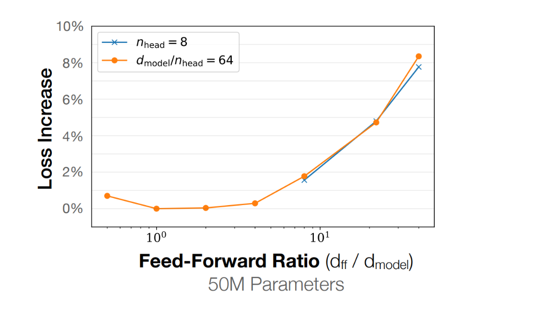
What can we learn from these hyperparameter studies? Extensive evidence shows: if not using GLU activation, you can default to a 4× multiplier; if using GLU, approximately 2.66× can be used. These settings work well for most modern language models. However, T5 once again proves you don't have to follow these rules — you can break conventions and freely choose, because no hyperparameter is an iron law; reasonable language models can be obtained under other hyperparameter configurations. Interestingly, this story has an intriguing follow-up: T5's improved version T5v1.1 adopted the more standard 2.5× GeGLU multiplier. This perhaps suggests the original team reassessed and believed they should dial back the 64× multiplier and choose a more conventional configuration, ultimately indeed obtaining a better model.

On the relationship between ratio and model efficiency: this ratio essentially controls the width of the MLP (FFN) hidden layer. The T5 paper's original rationale for choosing 64× was that maximizing this dimension enables larger matrix multiplications. While theoretically increasing width brings more parallel computation rather than serial computation, this actually represents a suboptimal allocation of parameters and computation at the cost of expressiveness — though when matrices are sufficiently wide, system performance gains may also be obtained.

4.3.2 Attention Heads and Model Dimension Ratio

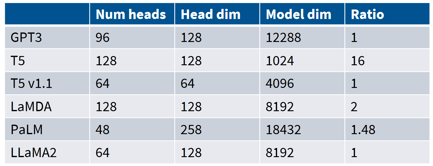
Another hyperparameter consensus is the ratio of model dimension to head dimension times number of heads. The standard approach is to keep per-head dimension fixed while increasing head count; alternatively, one could keep single-head dimension unchanged to increase the parameter count of the attention portion — but most models follow the former approach. Looking at GPT-3, T5, LaMDA, PaLM, and LLaMA 2, their ratios are all 1 or nearly exactly 1: $(NumHeads\cdot HeadDim)/ModelDim=1$. T5 is the sole exception breaking this rule, trying a ratio as large as 16. But aside from that, all other models quite closely follow this consensus.

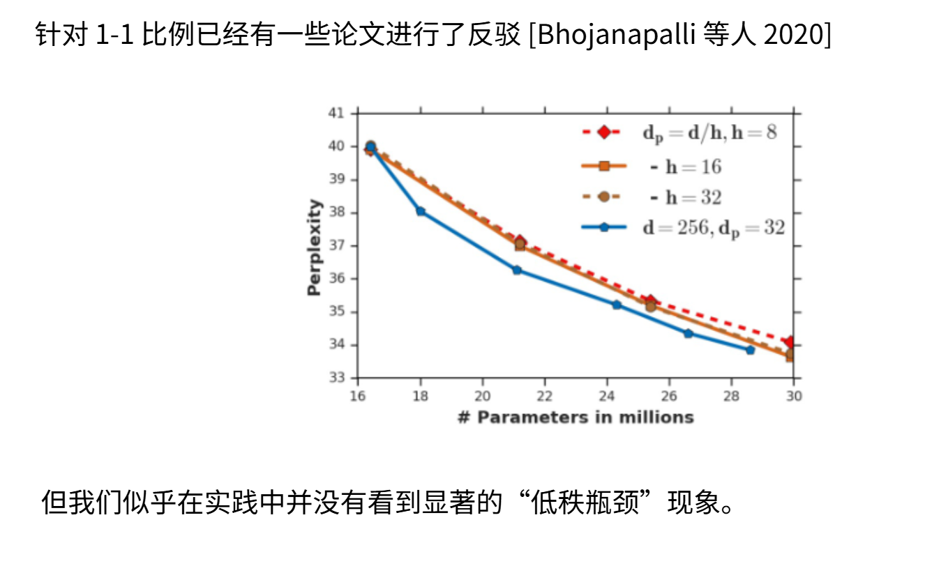
Bhojanapalli et al.'s 2020 study proposed that as the number of attention heads continuously increases, their rank becomes progressively lower. If per-head dimension is very small, it begins to affect the expressive power of the attention operation. But in practice, we don't seem to encounter many significant low-rank bottleneck issues. Most models adopting the 1:1 ratio perform very well.

4.3.3 Model Width-Depth Ratio

Should our model be deeper or wider? How deep and how wide?

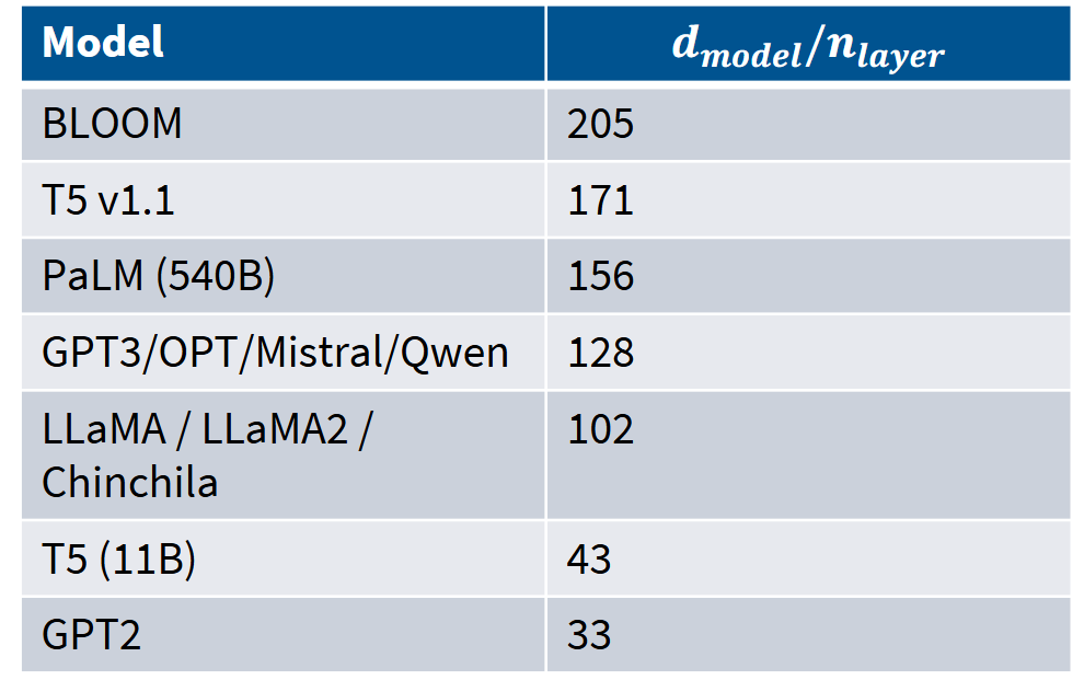
A widely applicable optimal criterion exists: each layer needs approximately 128 hidden dimensions. This standard is followed by many GPT-3 and LLaMA variant models.

The width-depth ratio consideration is very important — it controls the degree of parallelism we can achieve. If using pipeline parallelism, different layers are typically partitioned and assigned to different devices or device blocks, since each layer is also internally parallelized. This imposes specific constraints on the model. For particularly wide models, tensor parallelism can be used, distributing matrix slices across multiple GPUs. As we'll learn in subsequent chapters, different parallelism paradigms produce different constraints. Tensor parallelism requires very high-speed networks, while pipeline parallelism has somewhat lower requirements on network speed or latency. Therefore, network constraints may in turn influence width-depth decisions.

Setting aside these constraints, we can think abstractly: how does the width-depth ratio affect model performance? Kaplan et al. again provide excellent visualization. This shows three different data scales — 50M, 274M, and 1.5B parameters. The horizontal axis is the width-depth ratio, and the vertical axis is the percentage change in loss difference. We can see that around 100, a minimum appears across different scales.

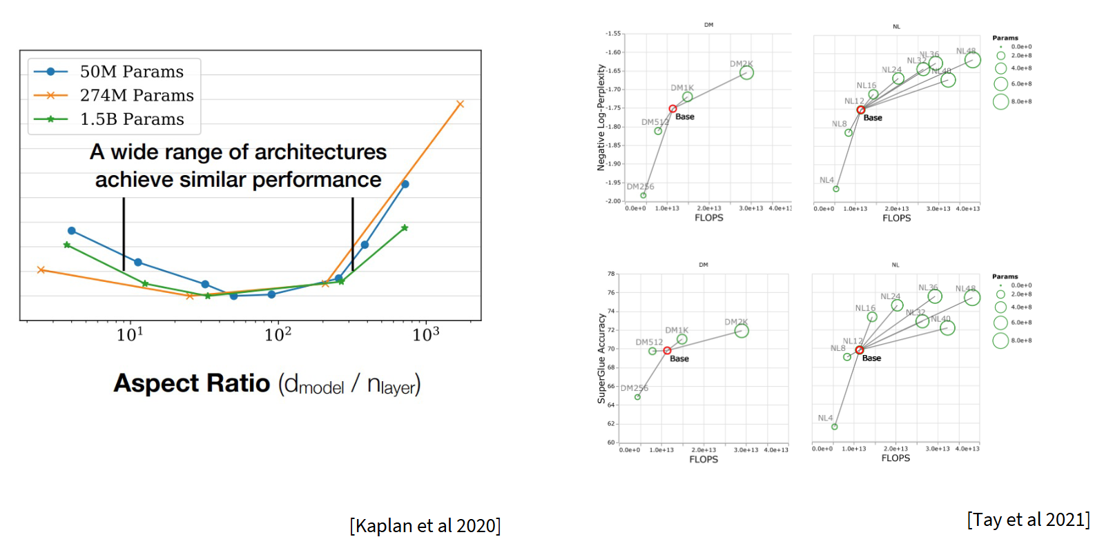
Google's ETay et al. have a very interesting study exploring the impact of depth versus width on upstream and downstream tasks. They found: if only looking at loss values, depth doesn't matter — parameter count is the sole critical factor. But when downstream accuracy is the evaluation metric, the picture becomes less clear. At the time, they were studying fine-tuned SuperGLUE accuracy. They believed that at the same computational cost (FLOPs), deeper models might perform better. There hasn't been much follow-up work on this. But from the perspective of aspect ratio, downstream task performance may indeed differ slightly.

Invisible Constraints of System Parallelism Strategies on Width-Depth Ratio

Beyond the optimal basin region in the loss function, the choice of width-depth ratio is also deeply influenced by parallelism strategies in invisible ways. Specifically:

Deeper models require partitioning across more layers, which typically forces the architecture to adopt Pipeline Parallelism. Pipeline parallelism has explicit "bubbles" and complex scheduling problems — challenges that system engineers strongly prefer to avoid. Wider models more easily use Tensor Parallelism, simply sharding a single large matrix multiplication across multiple GPUs, with more regular communication patterns and simpler implementation.

Therefore, the industry generally tends to moderately control depth while maintaining a certain width — in a sense, "trading system simplicity for training feasibility." This explains why actual large models rarely exhibit extremely deep or extremely wide designs, but mostly stabilize around a width-depth ratio of ~100 — this is the optimal compromise point among expressiveness, computational efficiency, and system engineering complexity.

4.3.4 Vocabulary Size

Overall, vocabulary size shows a continuously expanding trend. We believe this is largely because LLMs are being deployed in real production environments, gradually becoming more useful services. When this happens, models need to interact with people using different languages, process emoji and various near-modal or unexpected language forms. Early models (especially monolingual ones) typically had vocabularies in the 30K to 50K token range, such as early GPT and LLaMA series.

But observing multilingual models or what I call production-system models, their vocabularies have all expanded to the 100K to 250K range. Taking Cohere's Command model — which emphasizes multilingual processing — as an example, its vocabulary is very large. Even GPT-4 and its subsequent models using the GPT-4 tokenizer have vocabularies around 100K tokens. Therefore, 100K to 200K vocabulary has become the industry mainstream standard. Research shows that as model scale increases, models can to some degree handle more vocabulary elements and effectively utilize them. Thus, as model scale expands or training data increases, vocabulary size shows a continuously growing trend.

Q: Does a multilingual vocabulary help improve monolingual performance?

We believe multilingual vocabularies have minimal impact on high-resource languages (like English and Chinese). If only considering English language modeling, a smaller vocabulary works fine too. But where large vocabularies truly shine is in handling low-resource languages — not the tail of the data distribution, but more niche languages. A classic example is the models or tokenizers released by Cohere — they always emphasize that their large vocabulary design and tokenizer training approach enable non-English low-resource languages to be represented with fewer tokens, thereby dramatically reducing inference costs.

4.3.5 Dropout and Other Regularization Methods

Two important components that need to be set before the model runs: dropout and other regularization methods.

Pretraining appears to be the scenario least needing regularization — because pretraining typically only runs for one training epoch, and due to the enormous data volume, it's often impossible to even traverse all data. Single-epoch training makes overfitting nearly impossible. This seems to constitute sufficient reason for not needing regularization. But the actual situation is more complex. Early research heavily used dropout, and weight decay was also widely adopted. Although many teams no longer publish detailed training hyperparameters, dropout has gradually fallen out of favor, while weight decay continues to be used.

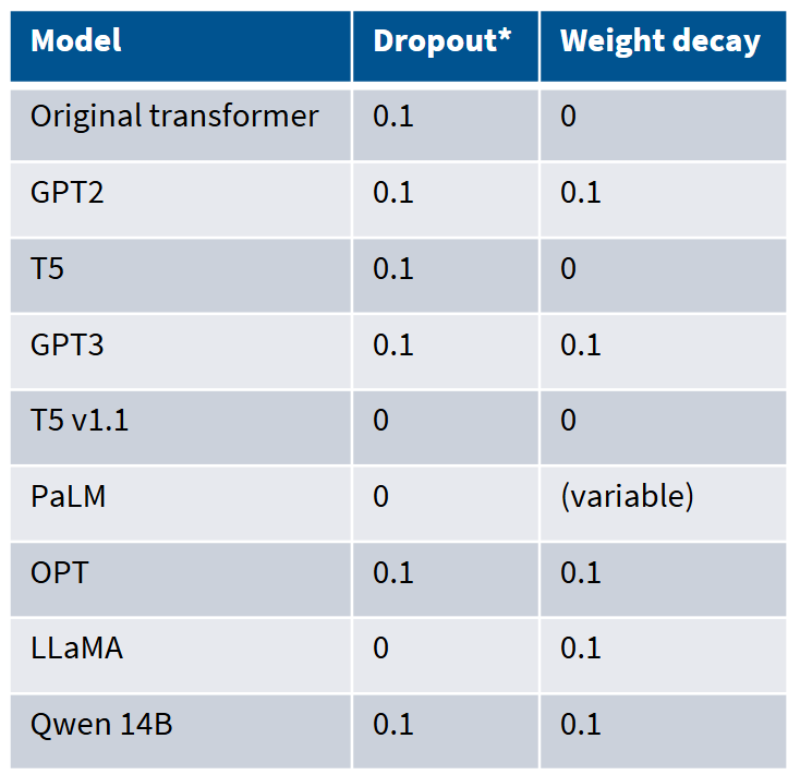
Many older models used dropout during pretraining; newer models (except Qwen) rely solely on weight decay.

This is actually quite paradoxical: when using SGD on massive data to train giant neural networks for a single epoch, why use weight decay?

The answer may be counterintuitive: weight decay is not used to control overfitting. Experiments show that different strengths of weight decay do not change the ratio between training loss and validation loss. Even with no weight decay at all, overfitting does not occur. What's truly interesting is that weight decay interacts with the optimizer's learning rate schedule in some peculiar way.

Implementing weight decay is not to regularize the model (though that was the original design intent), but to obtain lower training loss. This effect is achieved because at the end of training, as the learning rate approaches zero, various learning dynamics produce special effects. This is a very interesting, complex, and to some degree troubling property of language models. But now you should understand why many technical reports note "we used weight decay."

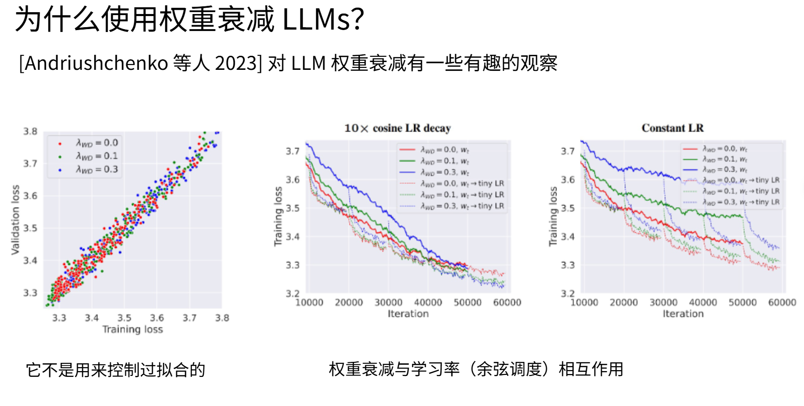
Now let's look at the different types of weight decay that can be implemented. When using weight decay, the model trains poorly at higher learning rates. When you lower the learning rate, the loss value drops rapidly. Observing cosine learning rate decay reveals that models with high weight decay progress slowly initially, but as the learning rate decreases (i.e., the cooling process), they optimize quickly. This indicates complex interactions between the optimizer and weight decay — at the end of training, some form of implicit acceleration occurs, ultimately producing a better model.

The True Role of Weight Decay: Regularizer or Optimization Accelerator?

A profound counterintuitive fact: in today's large-scale language model pretraining, Weight Decay almost no longer plays the regularization role of "preventing overfitting." Since data scale far exceeds the model's single-pass traversal capacity, overfitting simply doesn't occur — training loss and validation loss are highly consistent.

However, extensive experiments (such as Andriushchenko et al.'s research) show that appropriate weight decay can significantly reduce final training loss. Its mechanism is tightly coupled with the optimization process: at the end of training, when cosine learning rate decays to extremely small values, weight decay interacts complexly with optimization dynamics, producing some form of "implicit acceleration" that helps the model converge to better local minima. Therefore, weight decay is essentially an optimization intervention tool, not a regularization tool in the traditional sense. This also explains why, even under zero overfitting risk, nearly all modern large model training still retains weight decay.

---

4.4 Model Stability

The core architecture hasn't changed much over the past year, but many releases have prominently highlighted what are called stability techniques. These techniques aim to train models in a more stable manner. As model scale continuously expands and training time keeps extending, such stability issues become increasingly prominent.

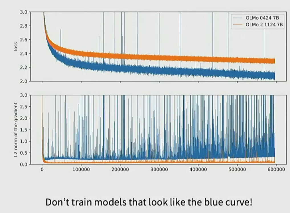
We can see this case from the OLMo 2 paper, which provides excellent academic work on LLM training stability. They first show this chart: observe the blue curve here — the L2 norm of this gradient plot is shocking. Although the loss curve appears normal, it occasionally exhibits anomalous spikes. Opening the gradient norm plot reveals a terrifying image full of spikes, with norm values completely out of control.

Training a model this way makes it very difficult to achieve reasonable convergence — ultimately, gradient norm explosion causes training to completely break down. Therefore, the current focus is how to transform the blue curve into something resembling the orange curve. Although the orange curve's loss value is higher (possibly due to dataset switching), its gradient norm consistently stays at the desired low level — this is the picture we want to see. So which parts of the Transformer are prone to causing stability issues? Actually, any part can be problematic, but based on existing technical interventions, one component truly stands out as the "problem child" — the softmax function. The root of the problem: exponential operations can cause numerical anomalies, and division operations can produce division-by-zero errors. For multiple reasons, softmax is indeed prone to various issues. It should be added: Transformers contain two softmax modules: one is the output layer softmax, and the other is the softmax within the self-attention mechanism.

Of the two softmax modules in Transformers:

• Self-attention softmax: when computing attention weights, logits ($Q{K}^T$) may become too large, causing gradient vanishing
• Output layer softmax: when generating distributions, logits may explode, making cross-entropy loss unstable

4.4.1 z-Loss Technique — Solving Output Layer Softmax

z-loss is a softmax normalizer regularization technique, formally proposed and named by Google in the PaLM model, though the idea can be traced back to earlier machine translation research. Its core goal is to prevent the softmax denominator (normalization factor Z) from becoming too large or too small, thereby stabilizing the training process.

$${\mathcal{L}}_{\text{z-loss}}=\lambda \cdot {\log }^{2}Z$$

where:

$Z$: the softmax normalization factor (partition function), $Z=\sum _{i=1}^V\exp (z_i)$

$\lambda$: weight coefficient (PaLM uses ${10}^{-4}$)

$z_i$: logits (unnormalized prediction scores)

Total loss function:

$${\mathcal{L}}_{\text{total}}={\mathcal{L}}_{\text{cross-entropy}}+\lambda \cdot {\log }^{2}Z$$

Its purpose is to keep the softmax normalizer within a good range. When z(x) is close to 1 (or log z is close to 0), the softmax can be considered in a good state. In a sense, PaLM was truly the pioneer. They were the first to use the z-loss trick, while many other models didn't adopt it for a long time — at least models with publicly available papers. However, a series of follow-up studies later emerged; as far as I know, the earliest follower was Baichuan 2, followed by DCLM, OLMo 2, and other models also adopting z-loss. This is a very elegant and practical stability improvement solution.

4.4.2 Solving Attention Layer Softmax Stability

$\text{Attention}(Q,K,V)=\text{softmax}\left(\frac{Q{K}^T}{\sqrt{d_k}}\right)V$

Standard flow:

$Q=W_q(x)$

$K=W_k(x)$

$logits=Q{K}^T/\sqrt{d_k}$

First pass query and key vectors through a LayerNorm layer:

$Q=\text{LayerNorm}(W_q(x))$

$K=\text{LayerNorm}(W_k(x))$

$logits=Q{K}^T/\sqrt{d_k}$

Before performing the softmax dot-product operation, first pass the query and key vectors through a LayerNorm layer. This is another approach to controlling softmax behavior — not controlling the normalization factor z, but controlling the numerical range of softmax inputs to naturally suppress undesirable behavior. As I mentioned earlier, this was initially an innovation in the vision and multimodal model domain: Dehghani et al.'s 2023 paper on training very large vision transformers first proposed it; subsequently, HuggingFace's Chameleon and Idefics adopted this trick in multimodal training components; now Gemma 2, DCLM, OLMo 2, and other models also use this technique to stabilize training.

Among stability interventions, the most surprising is the astonishing effectiveness of LayerNorm. We've witnessed LayerNorm evolve from only appearing at the front of modules, to covering both ends of non-residual components, and now extending into the Q and K components. At least in terms of improving stability, LayerNorm demonstrates remarkable effectiveness with almost no performance impact.

LayerNorm is applied during training. During inference, LayerNorm is still retained. Because LayerNorm has already learned parameters — its complete function is to normalize activations, then scale them by a specific factor. If this step were removed, it would cause a massive change to the model; the model would be unable to process those unnormalized activations.

4.4.3 Method 3: Soft Clipping of Logits Input to Softmax

Soft-clipping, also known as logit-capping or tanh-scaling, is an emerging softmax stabilization strategy. Its core idea: after the dot-product operation and before softmax, dynamically compress the extreme values of logits through the tanh function, keeping them bounded.

Standard Scaled Dot-Product

$$logits=Q\cdot K^T/\sqrt{d_k}$$

Possible range: $(-\mathrm{\infty },+\mathrm{\infty })$

Soft Clipping (adopted by Gemma 2/OLMo 2)

cap = 30.0 (soft clipping threshold)

$$logitsClipped=cap\cdot \tanh (logits/cap)$$

Range: $(-cap,+cap)$

After completing the dot-product operation in the self-attention mechanism, pass it through the soft-clipped softmax function. Specifically, use the formula above: taking logits as input, divide by the soft clipping value inside, multiply by the soft clipping value outside.

When your logits substantially exceed the soft clipping value, the tanh function clips them to 1. This way, you obtain the upper bound of the soft clipping value here. In some sense, this method achieves soft clipping of logits. Both Gemma 2 and OLMo 2 adopt this technique, though it hasn't become particularly popular yet.

Counter-evidence against this method comes from the previously mentioned NVIDIA team, who tried various stability-improving interventions. The study found: the baseline model's perplexity is 11.19; using soft clipping actually makes it worse, while QK normalization improves performance because it allows more aggressive learning rates, letting the optimizer play a greater role.

4.5 Summary

LLM architectures are constantly evolving. Many of the hyperparameters we set are based on empirical evidence or extensive experimental validation proving their utility. Drawing on the latest research findings and predecessors' experience, we can quickly retrofit a model — as simple as building with blocks.

Many aspects of the Transformer (architecture, hyperparameters) are similar across large language models.