Chapter 7: GPU High-Performance Programming

Learning Objectives

Before diving into specific analysis, let's clarify this section's focus. This section covers the core methods and practices of GPU high-performance programming:

1. Review GPU hardware architecture (SM, Warp, Block, Thread) and execution model, understand arithmetic intensity, thread block scheduling and other foundational concepts
2. Master benchmarking and profiling methods, learn to use PyTorch's built-in profiler and professional tools like Nsight Systems to locate performance bottlenecks
3. Deeply understand the principles of Kernel Fusion, and through hands-on CUDA kernel writing vs. Triton implementation comparison, experience the performance improvements from manual optimization to high-level abstraction
4. Learn to use Triton for writing efficient GPU kernels, understand its block-centric programming model, and compare performance with native PyTorch and hand-written CUDA
5. Understand torch.compile's automatic optimization capabilities and applicable scenarios, clarify when it's worth hand-writing low-level kernels vs. relying on the compiler

After completing this chapter, you will be able to: systematically master the complete workflow of GPU performance analysis and optimization, from benchmarking and profiling to kernel fusion and Triton programming; independently implement efficient GPU kernels for simple operators; and reasonably权衡 the use cases of hand-written optimization vs. compiler automatic optimization, thereby significantly improving computational efficiency in actual LLM training and inference tasks.

7.1 Review: GPU Architecture and Execution Model

7.1.1 GPU Hardware Architecture (A100/H100 as Examples)

Taking A100 or H100 as examples, GPUs contain many Streaming Multiprocessors (SMs), each SM internally has numerous processing units for executing computations, such as Int32 or FP32 units. Each SM launches large numbers of threads. The memory hierarchy includes large-capacity but slow DRAM (global memory), as well as faster caches. Pay special attention to the register file — this is extremely high-speed storage accessible per thread, and we will use these registers extensively when writing high-performance GPU code today.

Basic Structure of the Execution Model

The previous chapter covered Blocks, Warps, and Threads — in order of progressively finer granularity. A Block is a large thread group — each Block is assigned to one SM for processing. You can think of each SM as an independently working unit, and the Block as the processing unit assigned to it. Within each Block are many threads, each representing a task unit to be executed. These threads run in groups during execution — this grouping is called a Warp. Each Warp consists of 32 consecutively numbered threads, extracted from the Block for synchronous execution.

Block

Thread Block collections are scheduled onto a single SM for execution — this is the fundamental unit we need to focus on when programming in Triton and similar frameworks. Each Block contains many threads that actually perform computation. When operating on vectors, we have each thread simultaneously process code for multiple elements in the vector — all threads collaboratively complete the entire vector's processing. This is why we use Blocks rather than a global context.

Using Blocks enables efficient communication, because threads within a Block can exchange data through the SM's high-speed shared memory. For example, when matrix multiplication requires data passing between threads, intra-Block communication is extremely fast (comparable to L1 cache speed), while cross-Block communication is prohibitively expensive. Therefore, we should keep data within the same thread Block (or same compute unit) whenever possible to achieve high-speed performance. While thread synchronization within a Block is possible, cross-Block synchronization is not, and precise execution flow control is also impossible. Hence, we must avoid cross-Block communication.

SM (Streaming Multiprocessor)

Taking NVIDIA GPUs as examples (A100/H100/B200), SM counts across generations range roughly from 100 to 200, with modest variation. Each SM internally contains:

• Register File: B200 each SM has 65,536 registers, total capacity 256 KB. This count has been relatively stable across generations.
• L1 Cache / Shared Memory: Located inside the SM, size is on the same order of magnitude as registers (several hundred KB), with shared memory being explicitly controllable by the programmer.
• L2 Cache: Chip-level shared,容量 larger than L1 (tens of MB), accessible by all SMs.
• HBM (High Bandwidth Memory): Massive capacity (tens of GB), growing fastest across generations, but with the highest access latency.

In terms of bandwidth, there's essentially an inverse relationship: Registers > L1/Shared Memory > L2 > HBM. HBM bandwidth, while the slowest, still reaches TB/s levels (e.g., 8 TB/s). Key conclusion: Large-capacity memory (HBM) is slow but spacious; small-capacity memory (Registers, L1) is fast but limited in size.

Shared memory is divided into 32 banks, each bank 4 bytes wide. Within the same clock cycle, each bank can only serve one thread's access. If multiple threads within the same Warp access different addresses in the same bank, a bank conflict occurs, and accesses will be serialized. The worst case is a 32-way conflict (e.g., 32 threads simultaneously accessing the same column of data), causing severe performance degradation. Matrix multiplication data layouts need careful design to avoid this problem (mitigated through techniques like swizzling).

When 32 threads in a Warp access HBM, if the access addresses are consecutive and within a 128-byte cache line, these requests are merged into a single memory transaction (memory coalescing). This greatly improves bandwidth utilization. If thread access addresses are scattered (e.g., column-major access), it triggers multiple unnecessary transactions, causing effective bandwidth to plummet. This concept is similar to bank conflicts but operates at the HBM level.

Warp (Thread Warp)

A Warp is essentially a group of threads that execute together. The reason Warps exist is that these threads execute simultaneously — there's no need for separate control units per thread, just one per 32-thread block. So compute units far outnumber Warp schedulers. This enables more parallel work without worrying about control overhead. This is one of the GPU vs. CPU trade-offs: CPUs allocate more silicon area to control units and branch prediction, while GPUs emphasize compute capability with simplified control mechanisms.

Each Warp contains 32 threads. All threads within the same Warp must execute the same instruction in the same clock cycle (lockstep execution). If code contains branches (e.g., if cond: A else: B), and different threads within the Warp have different condition outcomes, these threads cannot simultaneously execute A and B. The hardware serially executes both paths: first letting some threads execute A (remaining threads wait), then letting remaining threads execute B. This control divergence severely reduces parallel efficiency, so branching should be avoided in GPU programming whenever possible.

When a Warp executes a high-latency operation (e.g., reading from HBM, potentially requiring hundreds of cycles), the SM's Warp scheduler immediately switches to another ready Warp with zero additional overhead. This means the SM can hide memory latency by concurrently running multiple Warps. As long as there are enough Warps available for switching, compute units remain busy. This is one fundamental reason GPUs need massive numbers of threads.

In actual execution, threads are grouped into consecutive 32-thread units (Warps), executing in batches on SMs. Therefore, we should strive to ensure all Warps have balanced computational load. Ideally, the number of thread Blocks should far exceed the number of SMs, and preferably be divisible by the SM count, so that each Warp's workload is balanced (each SM has its own Blocks to process, rather than idling). Empirically, the number of Blocks should be greater than 4× the number of SMs.

Occupancy and Register Pressure

Each thread can use at most 255 registers (hardware limit). The SM's total register count is fixed, so the more registers a single thread uses, the fewer threads/Warps the SM can simultaneously host, and the lower the occupancy. Thread Blocks are scheduled onto SMs for execution. If the total number of launched thread Blocks is not divisible by the SM count, then in the last batch of scheduling (tail wave), some SMs will be idle, wasting compute resources. Ideally, the total thread Block count should be an integer multiple of the SM count (or far greater than the SM count) to reduce this imbalance.

For example: a thread Block contains 128 threads, each thread uses 160 registers, so each Block needs 128×160 = 20,480 registers. If B200 each SM has 65,536 registers, that SM can simultaneously host at most 65,536 / 20,480 ≈ 3 thread Blocks, i.e., 3 × (128/32) = 12 Warps. B200 each SM can host at most 64 Warps, so Warp occupancy is 12/64 ≈ 18.75%. This low occupancy is caused by register pressure. But high occupancy is not always optimal — sometimes a trade-off with computational efficiency is needed.

For extremely lightweight element-wise operations, if each thread processes only one element, it generates massive numbers of threads with very little work per thread. We can use thread coarsening: have each thread process multiple elements (e.g., 8), thereby reducing total thread count, increasing per-thread computational intensity, while simplifying scheduling. Triton compiler's PTX output often automatically performs such optimizations.

Arithmetic Intensity

We should also introduce the concept of Arithmetic Intensity: FLOPs / bytes. If arithmetic intensity is high, the operation is compute-bound (good performance). Conversely, it's memory-bound (we want to avoid memory-bound situations).

In the previous chapter, we discussed that chip compute capability scales far faster than memory speed, so computation ultimately becomes limited by memory bandwidth, preventing full utilization of compute performance. Generally, matrix operations are compute-bound, while all other operations are memory-bound. So in GPU-related programming, we must minimize computation's dependence on memory as much as possible.

---

7.2 Performance Analysis Methods

The high-level principle for writing high-performance code is: must first benchmark and profile the code. Because students or developers often subjectively identify some part as the bottleneck, spend three hours optimizing it, only to discover it wasn't the bottleneck at all — wasting lots of time.

Using high-performance or fine-grained profilers allows accurate identification of bottleneck locations and the machine's actual operational state. Armed with this information, we can focus efforts on optimizing the most critical parts of code execution. This is the importance of this high-level philosophy, because specific methods about GPU execution details or how to write softmax kernels may continuously evolve, and we might even directly rely on the Torch compiler's automatic JIT functionality. But the importance of profiling will never change with tool evolution.

We hope everyone internalizes this concept: To write high-performance code, you must continuously profile.

7.2.1 Benchmarking

First, we define an MLP model, then generate random Gaussian-distributed input, and finally run for 5 steps, performing forward propagation then backward propagation each time, ultimately returning the mean of the MLP output. There's not even a loss function here — it's simply running MLP forward propagation and doing mean pooling at the end.

class MLP(nn.Module):
    """Simple MLP: linear -> GeLU -> linear -> GeLU -> ... -> linear -> GeLU and so on"""
    def __init__(self, dim: int, num_layers: int):
        super().__init__()
        self.layers = nn.ModuleList([nn.Linear(dim, dim) for _ in range(num_layers)])
    def forward(self, x: torch.Tensor):
        for layer in self.layers:
            x = layer(x)
            x = torch.nn.functional.gelu(x)
        return x

def run_mlp(dim: int, num_layers: int, batch_size: int, num_steps: int) -> Callable:
    # Define a model with random weights
    model = MLP(dim, num_layers).to(get_device())
    # Random Gaussian-distributed input X
    x = torch.randn(batch_size, dim, device=get_device())
    def run():
        # Run model `num_steps` times (note: no optimizer updates)
        for step in range(num_steps):
            # Forward propagation
            y = model(x).mean()
            # Backward propagation
            y.backward()
    return run

We'll run a simple multi-layer perceptron, with 128 dimensions, 16 network layers, specified batch size, and 5 training steps. Here we only execute forward and backward propagation 5 times each.

# Pseudocode for benchmarking (measuring runtime) and profiling (exploring time distribution within functions)

def benchmarking_and_profiling():
    run_mlp(dim=128, num_layers=16, batch_size=128, num_steps=5)
    benchmarking()       # How long does it take?
    profiling()          # Where is time being spent?

Next, we need to do two things: benchmarking (measuring runtime) and profiling (exploring time distribution within functions).

Let's start with benchmarking. Benchmarking is measuring the actual wall-clock time to execute these operations — here we only need to focus on the end-to-end execution time of the MLP function.

Our goal with benchmarking is to compare the performance of different implementations: comparing Triton implementation vs. hand-written C++, PyTorch implementation, and Torch compilation. We need to evaluate whether writing CUDA kernels is worthwhile, and also want to understand how much performance degrades when matrix multiplication scale increases. Therefore, we need empirical benchmarking.

This chapter will consistently use this benchmark function, which contains: the run function to test, several warmup iterations, and multiple正式 test iterations.

Warmup

The first time PyTorch code runs is much slower than subsequent iterations, because the first run involves initialization overhead like compiling code, sending instructions to GPU, etc. Warmup ensures we measure steady-state speed rather than startup speed. When running thousands or tens of thousands of iterations, what we care about is steady-state performance, not the speed of JIT-compiling CUDA code.

CUDA Synchronization

Another important point is calling torch.cuda.synchronize(). This is because GPU and CPU are two independent compute units that can run in parallel. Our Python code executes on the CPU — when running relevant computations, it dispatches CUDA kernels to the GPU, at which point the CPU continues executing subsequent code without waiting for GPU completion. While this特性 benefits writing high-performance code, it causes problems for benchmarking: if the GPU is asynchronously executing while the CPU runs other tasks, we cannot accurately measure GPU execution time, because GPU is computing offline, the CPU won't wait for GPU but continues executing code, causing timing to end prematurely.

torch.cuda.synchronize() ensures GPU and CPU reach a synchronized state, flushing all queued tasks so both are at the same code execution node. This enables us to perform multiple timing measurements in a truly synchronized state.

# Benchmarking code

def benchmark(description: str, run: Callable, num_warmups: int = 1, num_trials: int = 3):
    """Benchmark `func` by running it `num_trials`, and return all the times."""
    # Warmup: first run may be slower due to compilation and caching
    # We'll run the kernel multiple times because what matters is steady-state runtime.
    for _ in range(num_warmups):
        run()
    if torch.cuda.is_available():
        torch.cuda.synchronize()  # Wait for CUDA threads to complete (very important!)
    # Now actually time!
    times: list[float] = []
    for trial in range(num_trials):  # Multiple repetitions
        start_time = time.time()
        run()  # Actually execute computation
        if torch.cuda.is_available():
            torch.cuda.synchronize()  # Wait for CUDA threads to complete synchronization
        end_time = time.time()
        times.append((end_time - start_time) * 1000)
    mean_time = mean(times) # Average over multiple measurements
    return mean_time

Thus, if the CPU runs faster, it will wait for GPU execution to actually complete, and vice versa. Now we measure completion and take the average, because single measurements may fluctuate due to GPU thermal characteristics and other factors, hence need multiple repeated measurements, returning the average result.

This is our benchmarking code. Remember two key points: perform warmup, call CUDA synchronization. If you forget these, you may get extremely anomalous data (e.g., showing large matrix multiplication completing instantly, which is clearly impossible).

7.2.2 Matrix Multiplication Benchmarking

Now we can benchmark matrix multiplication. I'll progressively demonstrate partial results. Although we're just using data to verify known conclusions, I hope concrete demonstrations ensure consistent understanding. We'll run tests on the A100 GPU used in the course, measuring across different sizes of matrix multiplication, systematically collecting time consumption data across various dimensions.

    # Matrix multiplication benchmarking code

    '''
    Benchmarking measures the actual wall-clock time to perform some operation.
    It only gives you end-to-end time, not where time is spent (that's profiling).
    Compare different implementations (which is faster?), and understand how performance scales (e.g., as dimensions increase).
    '''

    benchmark("sleep", lambda : time.sleep(50 / 1000)) # Using the benchmark function implemented above
    
    if torch.cuda.is_available():
        dims = (1024, 2048, 4096, 8192, 16384)  # Different dimensions
    else:
        dims = (1024, 2048)
    
    matmul_results = [] 
    for dim in dims:
        result = benchmark(f"matmul(dim={dim})", run_operation2(dim=dim, operation=lambda a, b: a @ b))
        matmul_results.append((dim, result))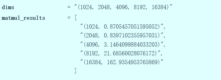

As expected, as matrix size increases, runtime shows super-linear growth. However, at the smallest sizes (like 1024 and 2048), time consumption barely grows, because executing matrix multiplication has fixed overhead: needing to transfer data from CPU to GPU, kernel launch overhead as well, so it doesn't maintain super-linear growth from absolute zero. But when matrices are sufficiently large, we indeed observe the expected scaling规律.

7.2.3 MLP Benchmarking

def benchmarking():
    
    # Test our MLP

    dim = 256
    num_layers = 4
    batch_size = 256
    num_steps = 2
    mlp_base = benchmark("run_mlp", run_mlp(dim=dim, num_layers=num_layers, batch_size=batch_size, num_steps=num_steps))
    

    # Below are basic scaling tests


    # Scale number of steps
    step_results = []

    for scale in (2, 3, 4, 5):
        result = benchmark(f"run_mlp({scale}x num_steps)", 
                         run_mlp(dim=dim, num_layers=num_layers, 
                                batch_size=batch_size, num_steps=scale * num_steps))
        step_results.append((scale, result))
    
    # Increase number of layers
    layer_results = []
    for scale in (2, 3, 4, 5):
        result = benchmark(f"run_mlp({scale}x num_layers)", 
                         run_mlp(dim=dim, num_layers=scale * num_layers, 
                                batch_size=batch_size, num_steps=num_steps))
        layer_results.append((scale, result))
    
    # Increase batch size
    batch_results = []
    for scale in (2, 3, 4, 5):
        result = benchmark(f"run_mlp({scale}x batch_size)", 
                         run_mlp(dim=dim, num_layers=num_layers, 
                                batch_size=scale * batch_size, num_steps=num_steps))
        batch_results.append((scale, result))
    
    # Scale dimensions
    dim_results = []
    for scale in (2, 3, 4, 5):
        result = benchmark(f"run_mlp({scale}x dim)", 
                         run_mlp(dim=scale * dim, num_layers=num_layers, 
                                batch_size=batch_size, num_steps=num_steps))
        dim_results.append((scale, result))

Now let's try benchmarking the MLP. The specific setup: scale MLP to 256 dimensions, set four network layers, batch size 256, execute two training steps. Measured time 6.2 seconds (mlp_base).

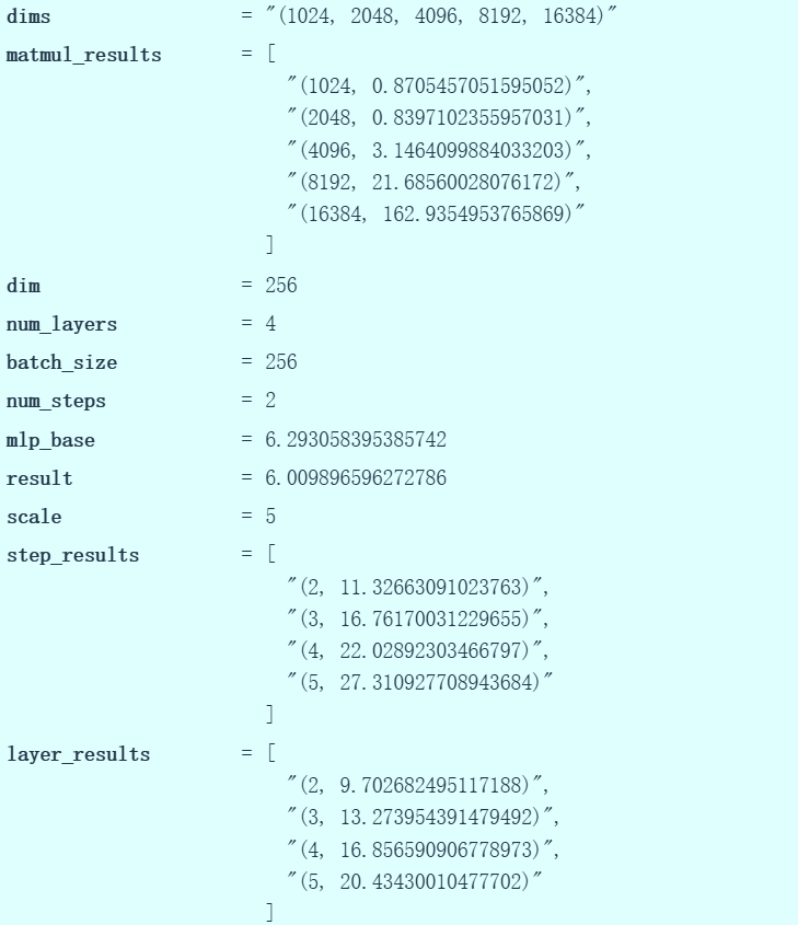
Next, we can perform basic scaling tests: gradually increase training steps from 2 to 5, benchmarking each. Unlike matrix multiplication, when increasing MLP forward and backward propagation count, runtime should grow linearly — actual data confirms this, with each MLP execution taking about 5 seconds, and overall runtime basically following the n×5 seconds pattern. Similarly, as network layers increase from 2, 3, 4 to 5, runtime also increases accordingly. Again, linear growth trend: single layer runs about 5 seconds (slightly less than 5), total time approximately 4× the layer count. Once again confirming linear scaling规律.

This完全 matches expectations — whether training steps or network layers, both have linear relationships with runtime. We'll skip the batch size scaling test since the tracked data volume is already somewhat excessive. So benchmarking stops here.

We created this benchmark function that performs a small number of warmups, executes CUDA synchronization, and can measure the runtime of any code we want. We can measure runtime of new architectures. But benchmarking is a coarse-grained measurement tool — it tells you code runs slowly, but cannot point out where exactly time is being spent. Therefore, we prefer using profiling, a more fine-grained measurement.

7.3 Profiling Tools

The profiling function structure is roughly as follows: similarly perform warmup, execute Torch CUDA synchronization, then invoke the profiler to simultaneously track CPU and GPU time. Next, run the target code, synchronize again, and output an average time table.

def profile(description: str, run: Callable, num_warmups: int = 1, with_stack: bool = False):
    # Warmup
    for _ in range(num_warmups):
        run()
    if torch.cuda.is_available():
        torch.cuda.synchronize()  # Wait for CUDA threads to end
    
    # Run code with profiler
    
    with torch.profiler.profile(
            activities=[ProfilerActivity.CPU, ProfilerActivity.CUDA],
            # Output stack traces for visualization
            with_stack=with_stack,
            # Need to export stack traces for visualization
            experimental_config=torch._C._profiler._ExperimentalConfig(verbose=True)) as prof:
        run()
        if torch.cuda.is_available():
            torch.cuda.synchronize()  # Wait for CUDA threads to end
    # Print table
    table = prof.key_averages().table(sort_by="cuda_time_total",
                                      max_name_column_width=80,
                                      row_limit=10)
    # Write stack trace visualization
    if with_stack:
        text_path = f"var/stacks_{description}.txt"
        svg_path = f"var/stacks_{description}.svg"
        prof.export_stacks(text_path, "self_cuda_time_total")
    return table

Profiling will be the more refined operation we need to perform. Profiling not only identifies which function time is spent in — we can view call stacks. Typically, we interact with the PyTorch interface layer, i.e., directly calling PyTorch components, but beneath PyTorch exists a complete CUDA invocation hierarchy. When running the profiler, we can trace all the way down to底层 calls, seeing the actual code path being executed. This provides more intuitive understanding of the program's真实 execution process on hardware. PyTorch has a very convenient built-in profiler tool. This lets us obtain clear output without leaving the Python or PyTorch environment. PyTorch has an excellent built-in profiler: https://pytorch.org/tutorials/recipes/recipes/profiler_recipe.html

7.3.1 Profiling a Sleep Function

Using this sleep function example — that sleep function.

def profiling():
    sleep_function = lambda : time.sleep(50 / 1000)
    sleep_profile = profile("sleep", sleep_function)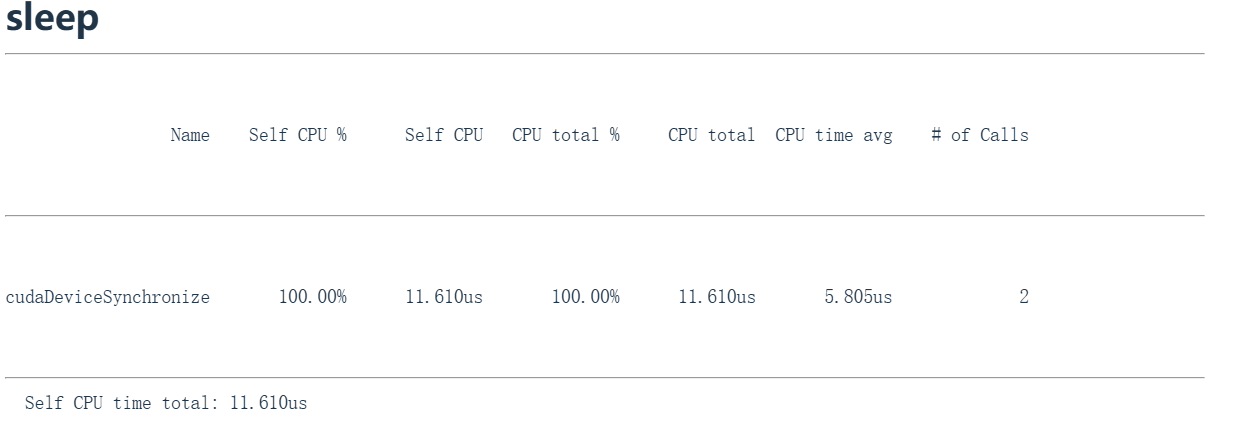

Observing the run results, we see 100% of time is spent on the operation called CUDA device synchronization (cudaDeviceSynchronize), because there are actually no GPU compute tasks. We're essentially profiling empty operations.

7.3.2 Profiling Matrix Addition

Now let's look at the following example with actual meaning. This is a basic matrix addition operation. First, we define an add function taking parameters A and B to perform matrix addition. This helper function instantiates two random Gaussian-distributed matrices and then calls the content in the operation parameter — adding two 2048-dimensional matrices.

def run_operation2(dim: int, operation: Callable) -> Callable:
    # Setup: create two random dim x dim matrices
    x = torch.randn(dim, dim, device=get_device())
    y = torch.randn(dim, dim, device=get_device())
    # Return a function to perform the operation
    return lambda : operation(x, y)

def profiling():
    add_function = lambda a, b: a + b
    add_profile = profile("add", run_operation2(dim=2048, operation=add_function))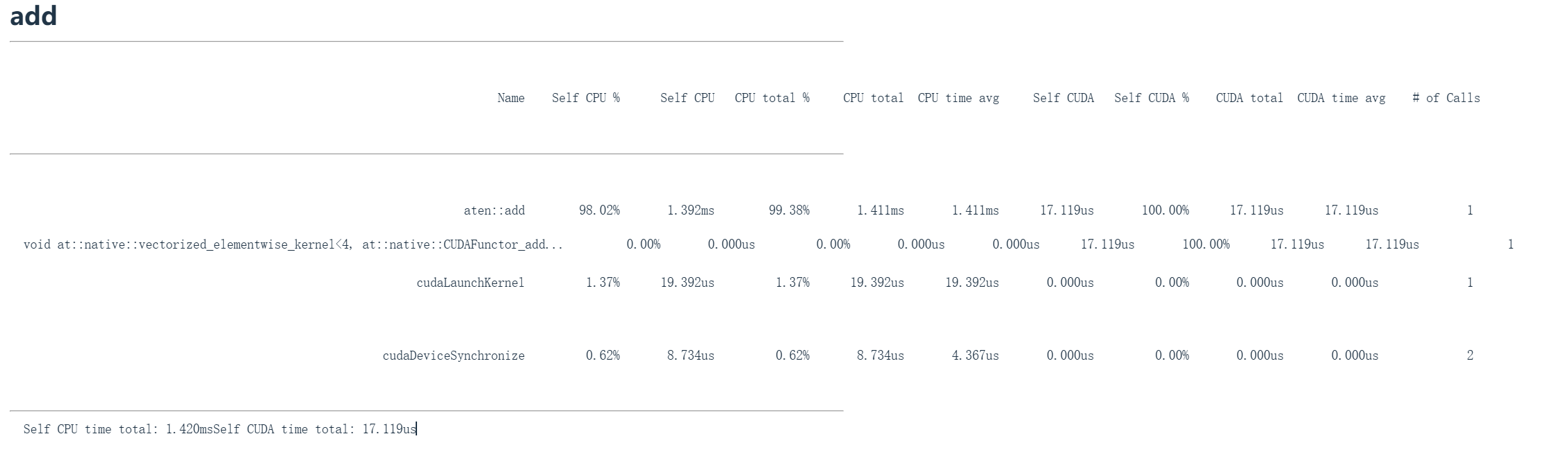

Now start profiling and calling the profiler — we'll get output similar to the image above. This is what the profiler returns.

When we call the add function in Python, the only thing we explicitly interact with is this add function — A plus B. But far more happens at the底层. This operation gets dispatched to the GPU for execution: first through aten:add (PyTorch's C++ interface layer, the second row in the table), this wrapper is called to confirm addition operation execution — this is the outermost invocation wrapper. Then it dispatches to the specific kernel function vectorized_elementwise_kernel4 (third row in the table), executing vector addition in nativeCUDA — this is where the actual addition happens. Simultaneously, CUDA kernel launch operations also consume time. CUDA kernel launch is essentially the CPU executing instructions and sending them to the GPU — i.e., kernel launch overhead. Finally, CUDA device synchronization needs to wait for GPU to complete computation and return data — this stage also consumes time. Just the synchronization operation itself consumes some time. Our final total time is: 1.4ms on CPU, 17µs on CUDA.

We can see GPU runs extremely fast while CPU is slower. Looking at CPU time (i.e., self CPU time), we find the C++ interface or C interface (like aten:add) actually consumes significant CPU time — these are overheads from transferring data to GPU. This is the internal execution mechanism of the add function.

7.3.3 Matrix Multiplication Profiling

def run_operation2(dim: int, operation: Callable) -> Callable:
    # Setup: create two random dim x dim matrices
    x = torch.randn(dim, dim, device=get_device())
    y = torch.randn(dim, dim, device=get_device())
    # Return a function to perform the operation
    return lambda : operation(x, y)


def profiling():
    matmul_function = lambda a, b: a @ b
    matmul_profile = profile("matmul", run_operation2(dim=2048, operation=matmul_function))

Matrix multiplication is a similar case. Here I perform A times B matrix multiplication, again using 2048-dimensional matrices for profiling. Now we see the aten:matmul call, indicating the底层 interface's matrix multiplication execution process. Then it calls Cutlass — NVIDIA's high-performance matrix multiplication CUDA library — subsequently dispatching to a specific Cutlass kernel containing tiling size parameters. This actually points to parameterized configurations like specific tile sizes and thread block counts — these are what execute matrix multiplication. Again at the bottom we see two familiar items: kernel launch (cuLaunchKernel) and CUDA device synchronization (cudaDeviceSynchronize). We can once again observe the distribution of CPU time vs. CUDA time. Since matrix multiplication is more time-consuming than vector addition, the CUDA portion's time share significantly increases.

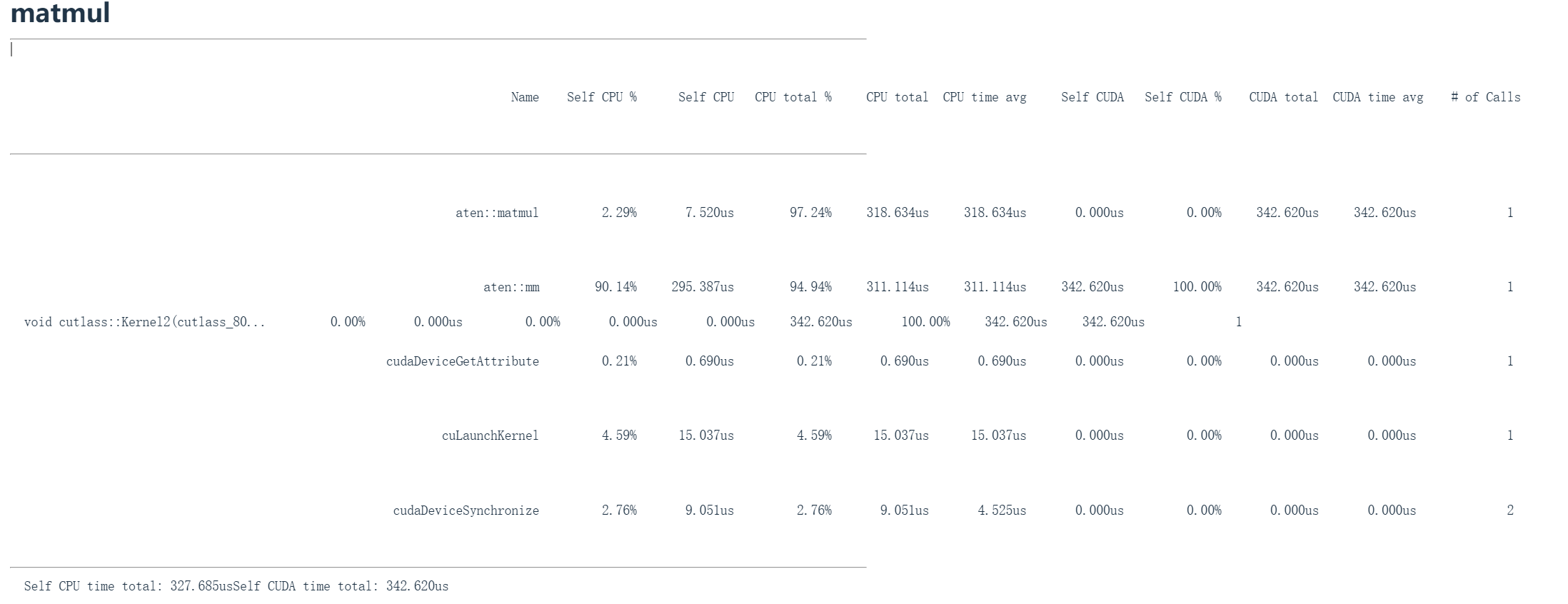
Here's another matrix multiplication example

def run_operation2(dim: int, operation: Callable) -> Callable:
    x = torch.randn(dim, dim, device=get_device())
    y = torch.randn(dim, dim, device=get_device())
    return lambda : operation(x, y)


def profiling():
    matmul_function_128 = lambda a, b: a @ b
    matmul_profile_128 = profile("matmul(dim=128)", run_operation2(dim=128, operation=matmul_function_128))

Here we multiply 128-dimensional matrices. 128×128 — much smaller than above.

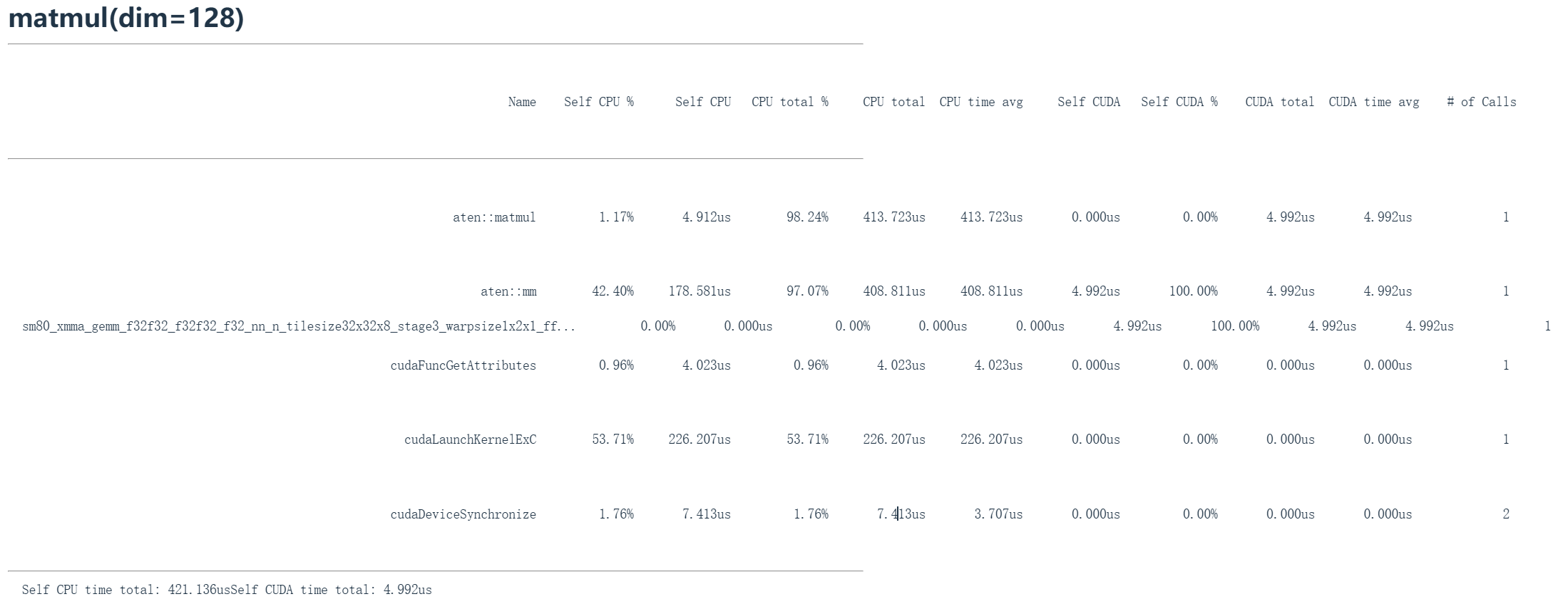
Through the kernel names output by PyTorch profiler, we can obtain substantial底层 implementation information. For example, the matrix multiplication kernel name cutlass_80_simt_sgemm_64x64x16:

• cutlass indicates use of NVIDIA's CUTLASS linear algebra library;
• 80 represents the SM architecture version (e.g., SM80 corresponds to A100);
• sgemm indicates single-precision general matrix multiplication;
• 64x64x16 is the tiling size.

For different matrix sizes, PyTorch may dispatch different kernels (e.g., for small sizes, it may directly use xmma_gemm bypassing CUTLASS). Understanding these names helps determine whether the optimal implementation is being used, and also allows leveraging torch.compile's auto-tuning feature to select the best kernel for your model.

You'll see it now directly executes this different command. From the line sm80_xmma_gemm_f32f32_f32f32_f32_nn_n_tilesize32x32x8_stage3_warpsize1x2x1_ff, we can see the difference from the matrix multiplication above — it executes xmma_gemm. GEMM is a type of matrix multiplication. Following is f32, i.e., float32. From this kernel's naming, we can see what's actually happening — this is a tiled matrix multiplication. It doesn't go through Cutlass but directly executes this specific command.

For small matrix multiplication, we see it now dispatches to a different kernel. This shows the complexity of matrix multiplication. When we operate at this high level of abstraction, we treat matrix multiplication as a single thing — we call A times B and it's done. But at the底层, depending on the dimensions and hardware you have, it actually dispatches to completely different matrix multiplication primitives. This manifests as截然 different performance characteristics. An interesting trick is torch.compile (which we'll cover later) — it actually has an option to macro-benchmark matrix multiplication performance on your hardware, then it selects the highest-performing matrix multiplication subroutine for your model. I've found this can带来 a free 10% speedup in the past. Optimizing these aspects brings free gains in reality.

The profiler's advancement over raw benchmarking is that we can now see which CUDA kernels are being invoked. We can see different matrix sizes lead to different CUDA kernels. We see cutlass_80simtt_sgemm from the Cutlass linear algebra library, which tells us tiling sizes and other information.

So far, these operations are relatively simple in some sense. Like matrix multiplication and addition. They're basically one-to-one: one operation on the CPU side translates to a GPU operation directly transferred over. We can do more complex operations.

7.3.4 Profiling torch.cdist — Complex Distance Computation

def run_operation2(dim: int, operation: Callable) -> Callable:
    x = torch.randn(dim, dim, device=get_device())
    y = torch.randn(dim, dim, device=get_device())
    return lambda : operation(x, y)


def profiling():
    cdist_function = lambda a, b: torch.cdist(a, b)
    cdist_profile = profile("cdist", run_operation2(dim=2048, operation=cdist_function))

This operation called torch.cdist computes pairwise Euclidean distances between vectors of two sets of matrices. This will be the large distance matrix computation between A and B that I need — this is cdist. This is a more complex operation: computing Euclidean distance requires computing dot products and also computing square roots.

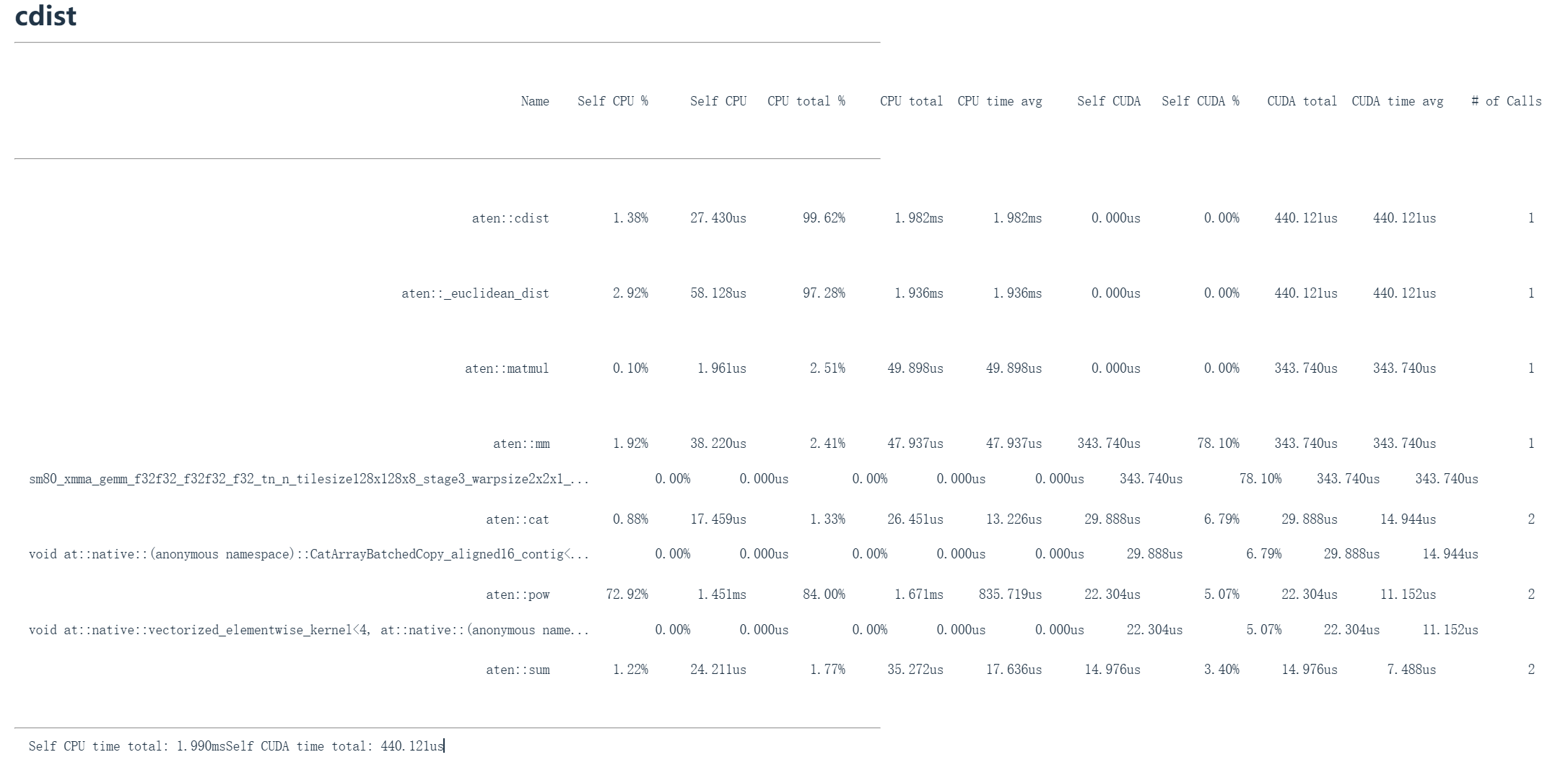
When we compute cdist, we see the image above — this is cdist's profiling output. We see this Torch Python command maps in the C interface to some lower-level cdist. The first row is aten::cdist, then maps to aten::euclidean_dist. Next, this decomposes into a whole set of operations: like aten::matmul, aten::pow, etc., because these are the basic primitives needed to compute Euclidean distances between all vectors.

When each matrix multiplication, concatenation, and power operation executes, there's a corresponding CUDA command being called here. We have the familiar GEMM — this is matrix multiplication, occupying 78% of GPU computation time. Then array copy and concatenation, occupying 6% of execution time. Then this vectorized element-wise kernel (performing power operations) takes 5% of GPU time, 3% for summation. Now we get a detailed breakdown of GPU time allocation.

From this, we know where to spend optimization time — for example, we could optimize matrix multiplication since it occupies over 70% of GPU time.

7.3.5 GELU and Softmax Profiling

def run_operation2(dim: int, operation: Callable) -> Callable:
    x = torch.randn(dim, dim, device=get_device())
    y = torch.randn(dim, dim, device=get_device())
    return lambda : operation(x, y)

def profiling():
    gelu_function = lambda a, b: torch.nn.functional.gelu(a + b)
    gelu_profile = profile("gelu", run_operation2(dim=2048, operation=gelu_function))

GELU is a nonlinear activation function. If you recall from Chapter 1, it's the Gaussian Error Linear Unit. It consists of products of tanh and exponential functions. We'll perform various operations: first execute A+B addition, then call the GELU function, simulating the linear-plus-nonlinear structure we might have in an MLP.

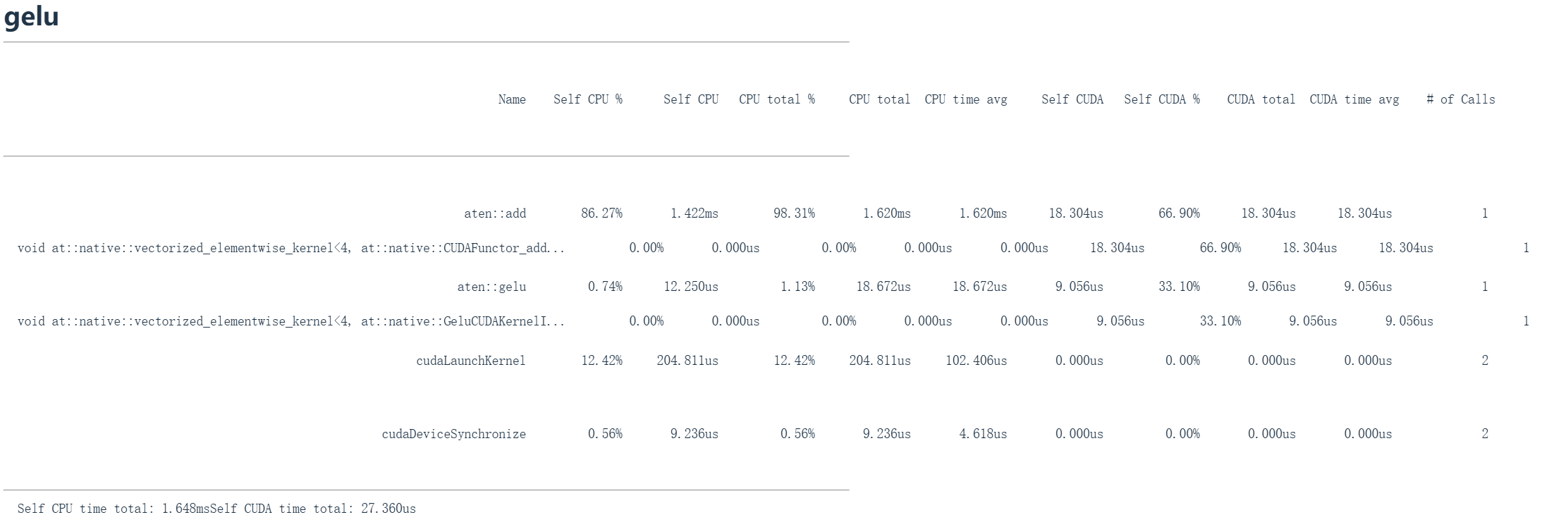
We again observe basically the same operation mappings — for example, aten::add corresponds to the A+B operation, then we see its CUDA equivalent implementation, and finally there's also a GELU function完全 implemented in CUDA, consuming about 33% of compute resources — a very reasonable proportion.

def run_operation2(dim: int, operation: Callable) -> Callable:
    x = torch.randn(dim, dim, device=get_device())
    y = torch.randn(dim, dim, device=get_device())
    return lambda : operation(x, y)

def profiling():
    softmax_function = lambda a, b: torch.nn.functional.softmax(a + b, dim=-1)
    softmax_profile = profile("softmax", run_operation2(dim=2048, operation=softmax_function))

Next, we see the softmax operation. Since these operation patterns repeat, I won't展开 detailed explanation for each one.

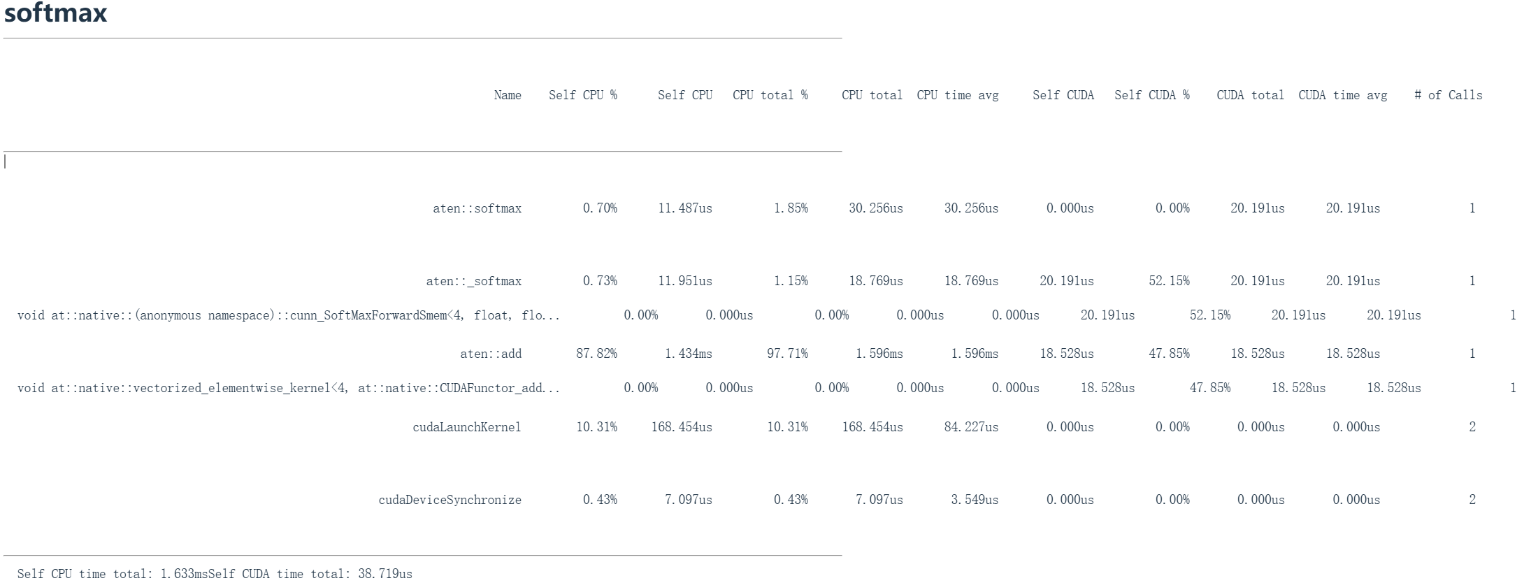
But the key subtlety worth emphasizing: core fundamental operators like softmax and GELU all have specially written kernel implementations. This means the GPU isn't executing basic primitive operations, but rather completing all computation at once through fused operators, completely avoiding round-trip data transfers between CPU and GPU (the operator fusion discussed in the previous chapter, which we'll also cover later in this chapter).

Now let's consider a more complex scenario. Take the MLP we initially used for benchmarking as an example — suppose we need to optimize this MLP for high-speed execution. Ideally, we need fine-grained profiling.

Using the Torch profiler produces results like this: recall the MLP structure's stacked linear layers, including forward and backward propagation processes. We can observe backpropagation-related operations, including matrix multiplication, linear operations, and gradient accumulation operations. Shown here (top to bottom) are matrix multiplication kernel implementations — the interface limits display to only 10 entries. Although the profiling results are truncated, we can still clearly see most time is spent on matrix multiplication operations.

However, in the self CUDA column, only 31% of time stays in the xmma module, while another 60% of time shows in aten::mm but without a corresponding kernel implementation — this appears somewhat mysterious. For complex modules, this kind of visualization isn't ideal.

7.3.6 Professional Profiling Tool: Nsight Systems

Now we can启用 a truly professional-grade profiling tool — NVIDIA Nsight Systems. This is NVIDIA's detailed GPU behavior and performance analysis solution, allowing us to precisely observe what actually happens during MLP execution.

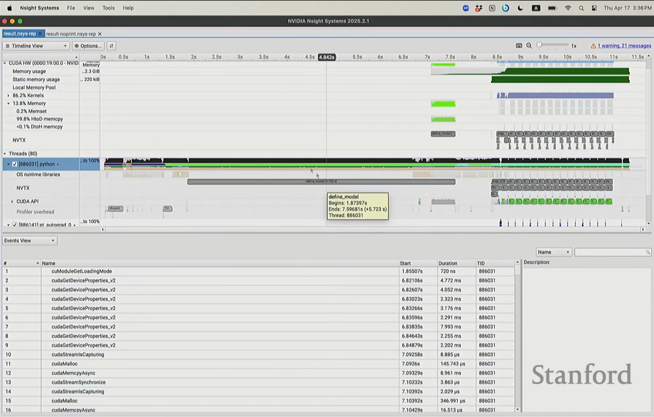
Essentially, when we observe profiling results, we see several different components. In the top-left panel, we can see the CUDA hardware section (CUDA HW), and below that, the Threads section. The upper CUDA region displays work being executed by the GPU. In the Threads section, we see tasks being processed by the CPU.

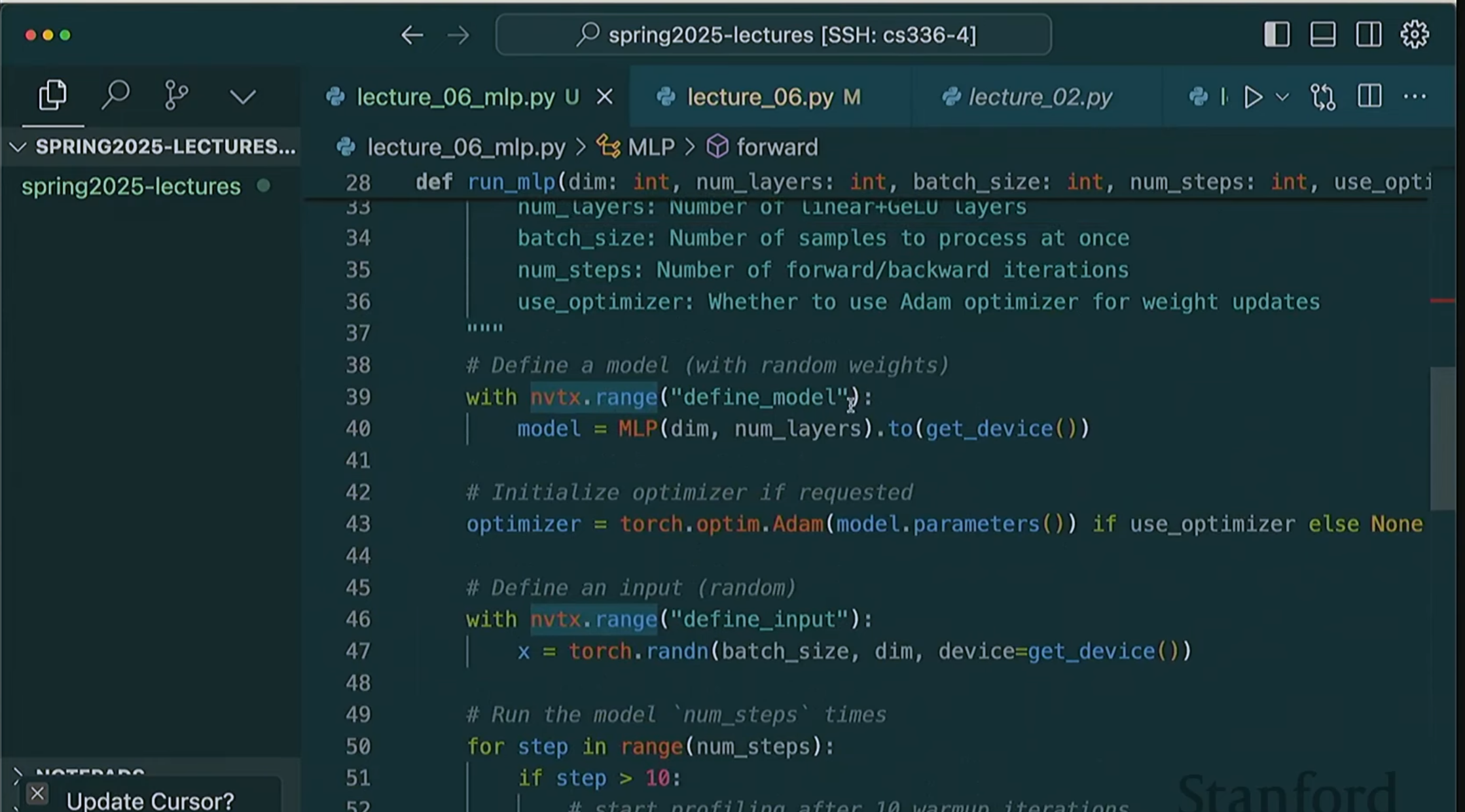
We can annotate code using NVTX tools, as shown in the figure above. This way, when the profiler runs, it can recognize that this code segment belongs to a code block named define_model (with nvtx.range("define_model"): model = MLP(dim, num_layers).to(get_device())).

Before invoking the profiler, we should have already added all these annotations in the code.

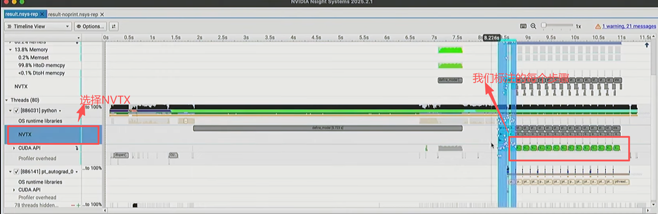
Operations like loading library files are very time-consuming — just initializing everything took 7.5 seconds. Then on the GPU side, the program only truly starts building the model after about 7.5 seconds of runtime.

The cooperation mechanism between CPU and GPU: the execution model works like this — when PyTorch code is first called, it doesn't execute directly but instead compiles code in real-time. Operations like module loading triggered at runtime are all overhead work from initializing layers and computation, moving code fragments into GPU — hence very time-consuming.

We can use this tool to see what happens at each step for both CPU and GPU — which operations consume time.

This software's operation is very complex and difficult to explain thoroughly in text and images. Due to space limitations, please refer to videos for learning.

---

7.4 Kernel Fusion

We introduced the concept of operator fusion in Chapter 6. Its core concept is avoiding round-trip data transfers between DRAM and SM for every operation, merging multiple operations into a single kernel.

GPU computation is like a small factory — each time an operation executes, data needs to be transported from warehouse to factory and back. If we sequentially execute a series of operations, it generates massive transport overhead from repeated warehouse trips. We want to build a factory that completes all operations at once, thereby avoiding data transport. Now we'll implement the GELU activation function and write kernel programs for it. We'll write this kernel in several different ways, then observe performance.

7.4.1 PyTorch and Manual Implementation of GELU Kernels

GELU's specific principles and details can be found in Chapter 4.

# PyTorch implementation of GELU

def pytorch_gelu(x: torch.Tensor):
    # Use the tanh approximation to match our implementation
    return torch.nn.functional.gelu(x, approximate="tanh")

This is the PyTorch-implemented GELU function, code as above. Calling torch.nn.functional.gelu with approximate=tanh parameter — this is to保持 completely consistent with the simple version we'll implement next. Here, we're not actually directly multiplying by the Gaussian cumulative distribution function, but using a more easily computable approximation.

Next, I'll demonstrate the manual implementation.

# Manual implementation

def manual_gelu(x: torch.Tensor):
    return 0.5 * x * (1 + torch.tanh(0.79788456 * (x + 0.044715 * x * x * x)))

You might look at this code and say: this performance must be terrible. We'll implement GELU in PyTorch like this: $0.5x(1+\tanh \left(0.79788456(x+0.044715x^3)\right))$. Although this formula looks complex, it approximates the GELU function. But implementing it this way involves many operations: hyperbolic tangent, cubic operations, constant multiplication, addition, and multiplication with 0.5 and x, etc. If these operations need to call multiple different CUDA kernels, execution efficiency will inevitably be low — this is the 直觉判断 we can make from the fusion concept.

# Run both implementations

    x = torch.tensor([1.])
    y1 = pytorch_gelu(x)
    y2 = manual_gelu(x)
    # Check if results match
    assert torch.allclose(y1, y2)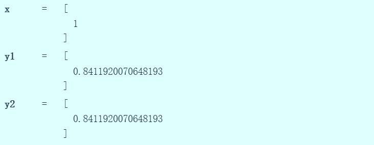

We can run the code and see the figure above showing both implementations produce identical computation results. If possible, you can systematically verify this on random Gaussian distributions.

Now benchmarking:

def run_operation1(dim: int, operation: Callable) -> Callable:
     # Create a dim x dim random matrix
    x = torch.randn(dim, dim, device=get_device())
    # Return a function to perform the operation
    return lambda : operation(x)

manual_time = benchmark("manual_gelu", run_operation1(dim=16384, operation=manual_gelu))
pytorch_time = benchmark("pytorch_gelu", run_operation1(dim=16384, operation=pytorch_gelu))

From the figure above, we see the manual implementation processing超大 data volume requires 8.1ms, while the PyTorch native implementation only needs 1.1ms.

7.4.2 Profiling Both Implementations

    # Profile both implementations

    manual_gelu_profile = profile("manual_gelu", run_operation1(dim=16384, operation=manual_gelu))
    pytorch_gelu_profile = profile("pytorch_gelu", run_operation1(dim=16384, operation=pytorch_gelu))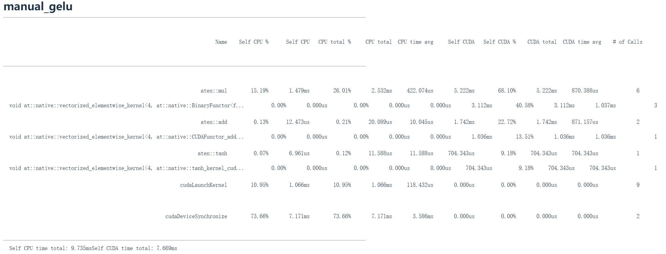

Now let's剖析 the underlying execution mechanism. The manual GeLU performs many operations — although vectorized, multiple CUDA kernels are launched here. Note the right side shows this CUDA kernel was called three times, because there are many floating-point multiplication operations, plus addition operations and hyperbolic tangent computation, where each operation may introduce latency (mostly communication overhead), ultimately leading to相当大的 time overhead.

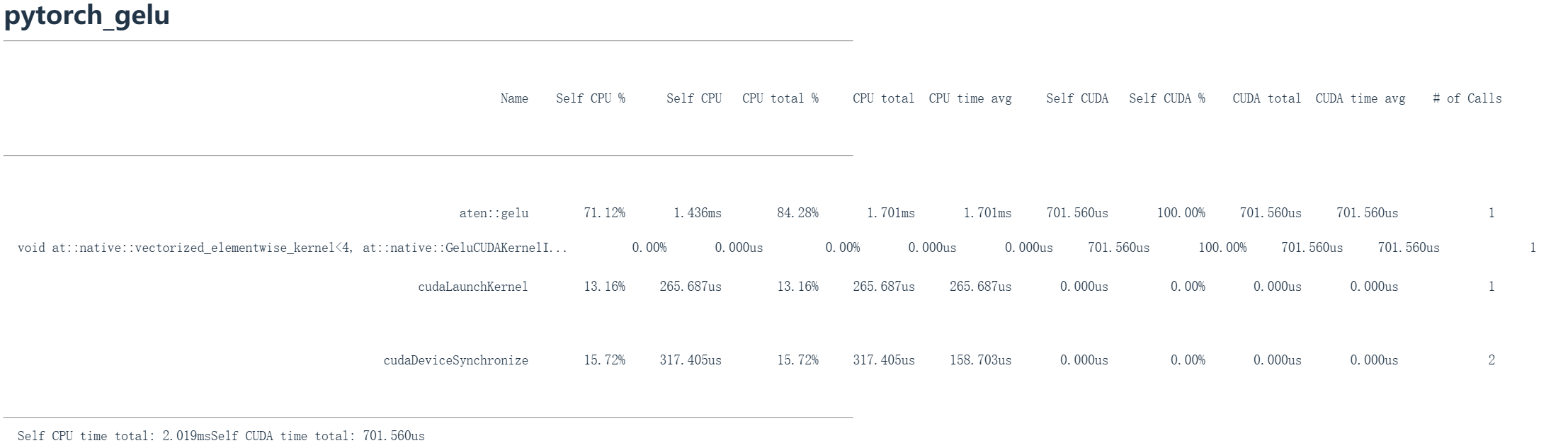
Now observe the PyTorch GELU implementation — just one CUDA kernel launch handles the entire task. This approach is very, very fast, because it launches only one CUDA kernel.

We hope to find a way to directly use CUDA kernels to achieve this. You might think the PyTorch team surely implemented this in the lowest-level language, so we should too. But we won't directly use the lowest-level language — however, we'll use the C++ API to write CUDA kernels.

7.4.3 Writing Kernels Using the C++ API

When we mention CUDA, we're actually referring to the C language API for interfacing with and programming GPUs. Based on the GPU logical model described earlier, we'll write a function f. When we call this CUDA kernel, it automatically executes function f on all elements of a vector or matrix, thereby achieving the parallel computation we need.

In terminology: we'll have a grid, which is a collection of thread blocks. Think of it this way: there's a task, split into several blocks. In a 2D grid, there are row and column coordinates — very useful when processing matrices. Each block has its dimensions, i.e., the number of thread blocks it contains — this is the block dimension. Each block internally contains a group of threads, forming a hierarchical structure: grid contains thread blocks, thread blocks contain threads.

Each function basically receives three parameters: block index (indicating which thread block it belongs to), block dimension information, and thread index. Through these parameters, we can determine our coordinates in the matrix or vector and execute the corresponding logic.

// File saved as gelu.cu, C++ CUDA code
// The Python code below uses cuda_gelu_src = open("gelu.cu").read() to invoke this code
#include <math.h>
#include <torch/extension.h>
#include <c10/cuda/CUDAException.h>


// Part 1: Kernel
__global__ void gelu_kernel(float* in, float* out, int num_elements) {
    int i = blockIdx.x * blockDim.x + threadIdx.x;
    if (i < num_elements) {
        out[i] = 0.5 * x * (1.0 + tanh(0.79788456 * (x + 0.044715 * x * x * x)));
    }
}

inline unsigned int cdiv(unsigned int a, unsigned int b) {
    return (a + b - 1) / b;
}

// Part 2: gelu function

torch::Tensor gelu(torch::Tensor x) {
    TORCH_CHECK(x.device().is_cuda());
    TORCH_CHECK(x.is_contiguous());
    torch::Tensor y = torch::empty_like(x);
    int num_elements = x.numel();
    int block_size = 1024;
    int num_blocks = cdiv(num_elements, block_size);
    
    // Launch kernel
    gelu_kernel<<<num_blocks, block_size>>>(x.data_ptr<float>(), y.data_ptr<float>(), num_elements);
    C10_CUDA_KERNEL_LAUNCH_CHECK();
    return y;
}

Now let's look at the GELU C++ code. This code has two parts: Part 1 above is gelu_kernel — this is the actual kernel responsible for computation work. It gets sent to the GPU to execute computation and return results. Part 2 is the gelu function — this is a wrapper running on CPU, responsible for coordinating kernel launch, while the kernel actually executes on GPU.

Part 1

Now let's look at the kernel itself: defined via __global__ void gelu_kernel(float* in, float* out, int num_elements), passing input/output pointers and element count. The __global__ keyword here identifies this as a CUDA kernel function.

Each thread needs to process a single element i, but the system doesn't directly tell the thread its coordinate position, so we need to compute it ourselves: int i = blockIdx.x * blockDim.x + threadIdx.x; — first get block index blockIdx.x (since this is 1D), multiply by block size blockDim.x to get the current block's starting position, then add thread index threadIdx.x, ultimately obtaining the global coordinate i. This coordinate computation pattern is common across all CUDA code.

Since there's no built-in bounds checking mechanism, we need to manually ensure processing stays within the valid range: by checking whether i is less than the total element count if (i < num_elements), letting end-position threads in memory-out-of-bounds positions execute nothing.

We execute the computation. Specifically, I'll do: out[i] = 0.5 * x * (1.0 + tanh(0.79788456 * (x + 0.044715 * x * x * x))); — get input data, access the i-th element via index, compute the gelu function the same way as before, assign the result to the i-th position of the output array — done.

Part 2

In the gelu function — these two key steps always need to be done in Triton or CUDA code. We always need to check two things: TORCH_CHECK(x.device().is_cuda()); TORCH_CHECK(x.is_contiguous()); — first, ensure input x is on a GPU device, e.g., some CUDA tensor. If not, problems arise because we can't do any computation on GPU. Second, we need to check ensure x is contiguously stored, because when we index into x, we'll perform many indexing operations where the system defaults to x being stored in contiguous memory blocks. If this condition isn't met, we can't achieve general-purpose processing — it must reside in contiguous memory blocks.

When computing gelu, we receive input x and need output y, so we need to allocate output space. Through torch::Tensor y = torch::empty_like(x), we create an output tensor space (or output tensor pointer) with the same dimensions as x. Note we don't call zeros here — this avoids extra operations since we'll overwrite this memory later — a small optimization worth implementing.

Next, we need to compute parameters: int num_elements = x.numel(); is total element count; int block_size = 1024; is the size of each block, i.e., how many threads per block; int num_blocks = cdiv(num_elements, block_size); is the total number of blocks needed.

When computing block count, we call the cdiv function — essentially dividing total elements by block size and rounding up, ensuring those final elements that can't be evenly divided by block size still get computed.

After completing this groundwork, we can launch the kernel. Through angle brackets, we specify block count and block size: <<<num_blocks, block_size>>> — these parameters get passed to the kernel instructions. Then we pass x and y pointers plus total element count: x.data_ptr<float>(), y.data_ptr<float>(), num_elements — these will be used to compute the kernel's boundary conditions.

In practice, memory几乎 never fragments because the system allocates contiguous memory space — unless you're doing very unusual operations (like transpose), non-contiguous situations don't arise. So when coding at higher levels, be aware: if you transpose then traverse something stored column-major, memory is no longer contiguous — there will be gaps between all elements during indexing. Block size depends on whether there are enough blocks to saturate the streaming multiprocessors, and whether each block has sufficient workload.

# Compile and run in Python
# CUDA is a C/C++ extension with APIs for managing GPU.
# Write f(i), CUDA kernel computes f(i) for all i.

# Grid: collection of thread blocks: numBlocks = (2, 4), blockDim = (1, 8)
# Thread block: collection of threads: blockIdx = (0, 1)
# Thread: single operation unit: threadIdx = (0, 3).
# You write code for threads to execute, using (blockIdx, blockDim, threadIdx) to decide what to do.

import os
import torch
from torch.utils.cpp_extension import load_inline

# Set debug mode so that CUDA tells you what went wrong if errors occur.
os.environ["CUDA_LAUNCH_BLOCKING"] = "1"


def create_cuda_gelu():

    cuda_gelu_src = open("gelu.cu").read()
    # The C++ code defines the gelu function

    cpp_gelu_src = "torch::Tensor gelu(torch::Tensor x);"
    # Compile the CUDA code and bind it to a Python module.
    ensure_directory_exists("var/cuda_gelu")
    if not torch.cuda.is_available():
        return None
    
    # `load_inline` makes it convenient to write CUDA code and bind it to a Python module for immediate use.  
    module = load_inline(
        cuda_sources=[cuda_gelu_src],
        cpp_sources=[cpp_gelu_src],
        functions=["gelu"],
        extra_cflags=["-O2"],
        verbose=True,
        name="inline_gelu",
        build_directory="var/cuda_gelu",
    )
    cuda_gelu = getattr(module, "gelu")
    return cuda_gelu

When debugging CUDA, set CUDA_LAUNCH_BLOCKING=1. This sacrifices some runtime performance but gives error message feedback. Otherwise, writing and debugging CUDA code would be very difficult.

Next, we can use load_inline to directly load our written CUDA gelu code and compile a Python module in the Python environment. Now that we've defined the CUDA function, we can call it directly in Python. We'll use C bindings to call this function. The CUDA gelu call is complete. I can verify that the manual gelu and CUDA gelu results are consistent.

Now let's benchmark both versions.

if cuda_gelu is not None:
    cuda_time = benchmark("cuda_gelu", run_operation1(dim=16384, operation=cuda_gelu))
    cuda_gelu_profile = profile("cuda_gelu", run_operation1(dim=16384, operation=cuda_gelu))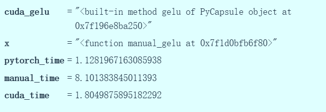

Here we record the time needed to run the PyTorch version — similar to the previous test result, approximately 1.1ms. The manual implementation time, remember, was 8.1ms.

Our CUDA version reduced the time to 1.8ms. Although not yet完全 reaching the PyTorch implementation's level, it's very close. Improving from 8ms to 1.8ms is pretty good progress, considering that C code wasn't complicated to write.

Now let's profile.

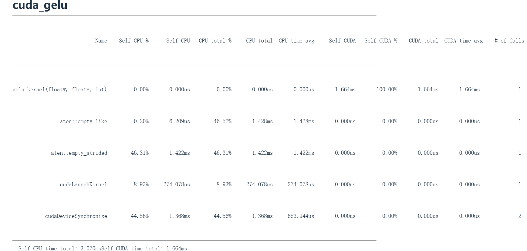
This shows the gelu_kernel kernel was called — this is the code sent to GPU for execution. Then aten::empty_like was called for initialization, followed by aten::empty_strided, then CUDA kernel launch and device synchronization operations.

In the Self CUDA column, this single CUDA kernel (gelu_kernel) occupies 100% of GPU time — this is the effect we want.

We fused all operators together, nicely solving the kernel fusion problem because we fused everything together, and the results are quite good. These types of element-wise operations are easy to implement in CUDA. If you need to implement some new nonlinear function, you完全可以 write the corresponding CUDA kernel yourself.

But more complex operations — for example, reduction operations requiring reading multiple values — are slightly more complex, just like implementing FlashAttention is harder.

Why is our manual implementation slower than writing a CUDA version? The CUDA version sends data from GPU back to CPU, then x will reside in GPU. In the manual version, we allocate it in GPU and process it similarly to the CUDA implementation, but it doesn't stay continuously in the streaming multiprocessor. So once we execute x squared, that's a CUDA kernel. This multiplication operation reads the vector from global memory into the streaming multiprocessor, executes computation, then writes back. So this is all DRAM-to-SM communication cost, not CPU-to-GPU communication cost. Of course, if it were a CPU device, there would be CPU transfer cost in addition to DRAM transfer cost.

Of course, we have better Python abstractions for writing CUDA kernels — namely, Triton.

7.5 Triton

Triton is a domain-specific language developed by OpenAI in 2021. It makes GPU programming more accessible because you don't need to manage all GPU details. Moreover, we can write everything in Python and no longer need to think about threads — instead, we think about thread blocks.

Triton manages many annoying but automatically optimizable things. It can manage memory coalescing. We covered burst mode in the previous chapter: you can fetch four adjacent values from DRAM at once. When you retrieve data from memory but it's grouped into calls of four adjacent elements or more, it handles this automatically.

When managing memory written by multiple threads within a streaming multiprocessor, it handles shared memory management. Within each SM, we sometimes need to stop or start threads — Triton can manage this automatically, but cross-SM scheduling or different SM operations are manual. So when using Triton, you'll think in terms of streaming multiprocessors, and the compiler will handle more底层 details.

A great aspect of Triton is that it can substantially outperform many PyTorch implementations. It's like directly writing CUDA within familiar Python territory — it's all in Python, and you can single-step debug.

7.5.1 Writing with Triton

Triton Implementation of Softmax (entire row fits in one block)

When one row of a matrix doesn't exceed the thread block size, an entire row can be assigned to one thread block. Triton code is almost identical to regular PyTorch, because intra-block operations automatically cover reduction and broadcasting.

@triton.jit
def softmax_kernel(x_ptr, y_ptr, n_cols, BLOCK_SIZE: tl.constexpr):
    pid = tl.program_id(0)          # Each block负责 one row
    row_start = pid * n_cols        # Starting address of this row
    offsets = row_start + tl.arange(0, BLOCK_SIZE)
    mask = offsets < (pid + 1) * n_cols  # Ensure no out-of-bounds

    x = tl.load(x_ptr + offsets, mask=mask, other=-float('inf'))
    x_max = tl.max(x, axis=0)       # Find max (numerical stability)
    x_exp = tl.exp(x - x_max)
    x_sum = tl.sum(x_exp, axis=0)
    y = x_exp / x_sum
    tl.store(y_ptr + offsets, y, mask=mask)

At launch, grid size equals row count. Each thread block independently completes that row's softmax computation — one read/write of HBM suffices, no cross-block communication needed.

---

Triton Implementation of Row Sum (data exceeds block size, requires tiled loop reduction)

When row length exceeds thread block size, we need to loop over multiple tiles within the block, each thread maintaining a local accumulator, with final cross-thread reduction.

@triton.jit
def row_sum_kernel(x_ptr, y_ptr, M, N, BLOCK_SIZE: tl.constexpr):
    pid = tl.program_id(0)          # Responsible for row pid
    row_start = pid * N
    acc = tl.zeros((BLOCK_SIZE,), dtype=tl.float32)  # Local accumulator

    for start in range(0, N, BLOCK_SIZE):
        offsets = row_start + start + tl.arange(0, BLOCK_SIZE)
        mask = offsets < row_start + N
        x = tl.load(x_ptr + offsets, mask=mask, other=0.0)
        acc += x                     # Accumulate current tile

    result = tl.sum(acc, axis=0)     # Cross-thread reduction sum
    tl.store(y_ptr + pid, result)    # Write scalar result back

Key points:

• The outer loop traverses tiles along the column direction, each time loading one tile's data and accumulating.
• After the loop ends, use tl.sum to complete inter-thread reduction, obtaining the row's sum.
• This intra-block loop + local accumulation + final reduction pattern is the core method for handling large rows (or more generally large dimensions), and is also the foundation for subsequent matrix multiplication tiling.

---

Triton Implementation of Matrix Multiplication (2D Tiling)

This is the most core operation in deep learning and the key case introducing two-dimensional tiling.

Problem with the naive implementation: If each thread computes one element of output matrix C, it must repeatedly read A's rows and B's columns from HBM — read/write count is O(M×K×N), low arithmetic intensity, limited by memory bandwidth.

Solution: Tile C, each thread block responsible for one C tile, loop along the K dimension loading corresponding A and B tiles into shared memory, perform local matrix multiplication within the block and accumulate. This way, each element only needs one read from HBM, arithmetic intensity提升 to O(tile_size).

@triton.jit
def matmul_kernel(A_ptr, B_ptr, C_ptr, M, N, K,
                  BLOCK_M: tl.constexpr, BLOCK_N: tl.constexpr, BLOCK_K: tl.constexpr):
    # Determine which C tile the current block is responsible for
    pid_m = tl.program_id(0)
    pid_n = tl.program_id(1)

    # Starting position of C tile
    offs_m = pid_m * BLOCK_M + tl.arange(0, BLOCK_M)
    offs_n = pid_n * BLOCK_N + tl.arange(0, BLOCK_N)

    # Accumulator, stored in shared memory / registers
    acc = tl.zeros((BLOCK_M, BLOCK_N), dtype=tl.float32)

    # Loop along K direction, loading A, B tiles
    for k in range(0, K, BLOCK_K):
        offs_k = k + tl.arange(0, BLOCK_K)
        # Load A tile [BLOCK_M, BLOCK_K], B tile [BLOCK_K, BLOCK_N]
        a = tl.load(A_ptr + offs_m[:, None] * K + offs_k[None, :])  # Need mask
        b = tl.load(B_ptr + offs_k[:, None] * N + offs_n[None, :])
        acc += tl.dot(a, b)   # Execute matrix multiplication within tile and accumulate

    # Optional: fuse activation function
    # acc = tl.maximum(acc, 0)  # relu

    # Write back C tile
    tl.store(C_ptr + offs_m[:, None] * N + offs_n[None, :], acc)

Key points:

• The grid is 2D, corresponding to C matrix's tile partition.
• Loop along the K dimension, each time loading a small block of A and B into shared memory (tl.load automatically utilizes shared memory).
• tl.dot executes efficient local matrix multiplication.
• Activation functions (like ReLU) can be fused before write-back, achieving operator fusion.
• Arithmetic intensity depends on BLOCK_K and BLOCK_M/N — larger tiles mean higher reuse rates, but are limited by shared memory size.

---

Implementing GELU

@triton.jit
def triton_gelu_kernel(x_ptr, y_ptr, num_elements, BLOCK_SIZE: tl.constexpr):
    # Input at `x_ptr`, output at `y_ptr`
    #     |        Block 0            |          Block 1          |      ...      |
    #                            BLOCK_SIZE                                 num_elements
    pid = tl.program_id(axis=0)
    block_start = pid * BLOCK_SIZE
    # Indices where this thread block should operate
    offsets = block_start + tl.arange(0, BLOCK_SIZE)
    # Handle boundary
    mask = offsets < num_elements
    # Read
    x = tl.load(x_ptr + offsets, mask=mask)
    # Approx gelu is 0.5 * x * (1 + tanh(sqrt(2/pi) * (x + 0.044715 * x^3)))
    # Compute (tl.tanh doesn't exist, use tanh(a) = (exp(2a) - 1) / (exp(2a) + 1)
    a = 0.79788456 * (x + 0.044715 * x * x * x)
    exp = tl.exp(2 * a)
    tanh = (exp - 1) / (exp + 1)
    y = 0.5 * x * (1 + tanh)
    # Store
    tl.store(y_ptr + offsets, y, mask=mask)

def triton_gelu(x: torch.Tensor):
    assert x.is_cuda
    assert x.is_contiguous()
    # Allocate memory for output tensor
    y = torch.empty_like(x)
    # Determine grid (elements divided into blocks)
    num_elements = x.numel()
    block_size = 1024  # Number of threads
    num_blocks = triton.cdiv(num_elements, block_size)
    triton_gelu_kernel[(num_blocks,)](x, y, num_elements, BLOCK_SIZE=block_size)
    return y

triton_gelu is the wrapper Triton GELU code — receives x, two assertions ensure x is on GPU and contiguous. Then uses empty_like to allocate an output tensor y. triton_gelu_kernel[(num_blocks,)](x, y, num_elements, BLOCK_SIZE=block_size) basically passes the same information to my kernel.

Now the Triton kernel is triton_gelu_kernel. This implements the same functionality as our earlier CUDA code, but now elegantly written in Python.

Input x_ptr will be at the x pointer location. Y pointer y_ptr is the output vector. BLOCK_SIZE represents the size of each block. num_elements will be the end position of my array.

pid = tl.program_id(axis=0)
block_start = pid * BLOCK_SIZE
offsets = block_start + tl.arange(0, BLOCK_SIZE)

These three lines compute indices. block_start = pid * BLOCK_SIZE computes the current block's starting position — block ID times block size. Then we need to know our position within the block; offsets will be the offsets. But note one difference: what we get isn't a single offset, because we're not programming threads — we're programming blocks. This means that actually my offset is a vector, not a single value. Because this is essentially performing vectorized operations, and vectorized operations will be handled by different threads. So here offsets = block_start + tl.arange(0, BLOCK_SIZE) — the offsets are the block's starting position plus a vector, i.e., this block_size offset range. In other words, my offset is the collection of all these coordinates within the block.

Of course, if at the very end, we might exceed the boundary, so we need a mask to handle all cases outside the vector boundary: mask = offsets < num_elements.

Now, I'll load all data at once through a single vectorized operation: x = tl.load(x_ptr + offsets, mask=mask). So x pointer plus offsets gives the values I want to process — after mask processing, loaded into x. This is the internal value we need, i.e., the internal temporary vector.

Using this temporary vector, I'll execute exactly the same GELU computation as before.

    a = 0.79788456 * (x + 0.044715 * x * x * x)
    exp = tl.exp(2 * a)
    tanh = (exp - 1) / (exp + 1)
    y = 0.5 * x * (1 + tanh)

There's no tanh function here, so we need to compute it manually. This formula is exactly the same as what we used before. Then y will be the result computed through the formula above. After completing computation, we need to write it back to the output buffer, i.e., the output vector: tl.store(y_ptr + offsets, y, mask=mask). So the computation target position is y pointer plus offsets in the parentheses, plus the temporary value y and mask. Then perform the store.

This is very, very similar to the earlier operations, but this is the vectorized version. We can operate on an entire block at once, so unlike thinking from a thread perspective, we now think from a block perspective — but the difference isn't large.

7.5.2 Triton Testing

    manual_time = benchmark("manual_gelu", run_operation1(dim=16384, operation=manual_gelu))
    pytorch_time = benchmark("pytorch_gelu", run_operation1(dim=16384, operation=pytorch_gelu))
    cuda_time = benchmark("cuda_gelu", run_operation1(dim=16384, operation=create_cuda_gelu()))
    triton_time = benchmark("triton_gelu", run_operation1(dim=16384, operation=triton_gelu))
    triton_gelu_profile = profile("triton_gelu", run_operation1(dim=16384, operation=triton_gelu))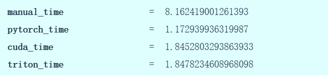

Manual GELU takes 8.1ms, PyTorch version 1.1ms, CUDA version 1.84ms, Triton version 1.848ms. Although speed hasn't improved, writing Triton code is much easier. We write in Python, think about block operations, and can do vectorized addition. If handling more complex tasks, Triton handles many memory operations for you — this is really nice.

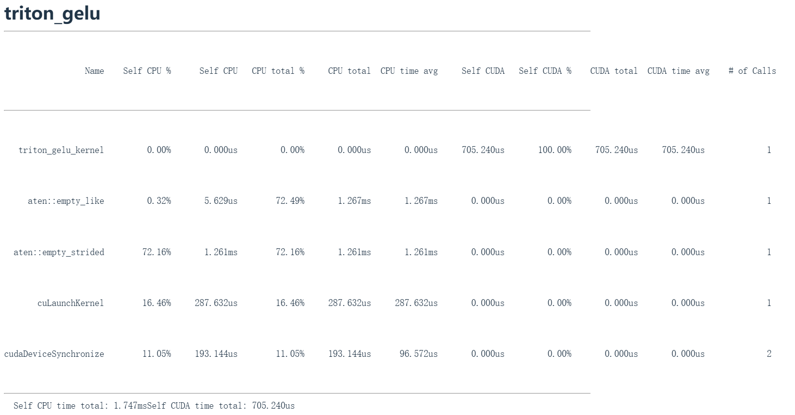
Profiling again shows that a single kernel launch consumes all GPU time — exactly what we want.

7.6 torch.compile

def pytorch_compilation():
    compiled_gelu = torch.compile(manual_gelu)
    check_equal(compiled_gelu, manual_gelu)
    if not torch.cuda.is_available():
        return

Writing CUDA kernels is nice, but perhaps we don't need to do so, because the tool torch.compile can achieve automatic optimization. What we do is stuff the cubic and exponential operations into a single CUDA kernel (compiled_gelu = torch.compile(manual_gelu)). torch.compile can take unoptimized PyTorch code and generate optimized versions. It attempts automatic kernel fusion and other optimizations. This compiled gelu produces results equivalent to the original. It essentially leverages PyTorch's existing JIT compiler to automatically optimize code.

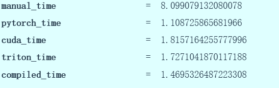
Now looking at runtimes: manual 8.1ms, PyTorch 1.1ms, CUDA 1.8ms, and torch.compile only needs 1.47ms.

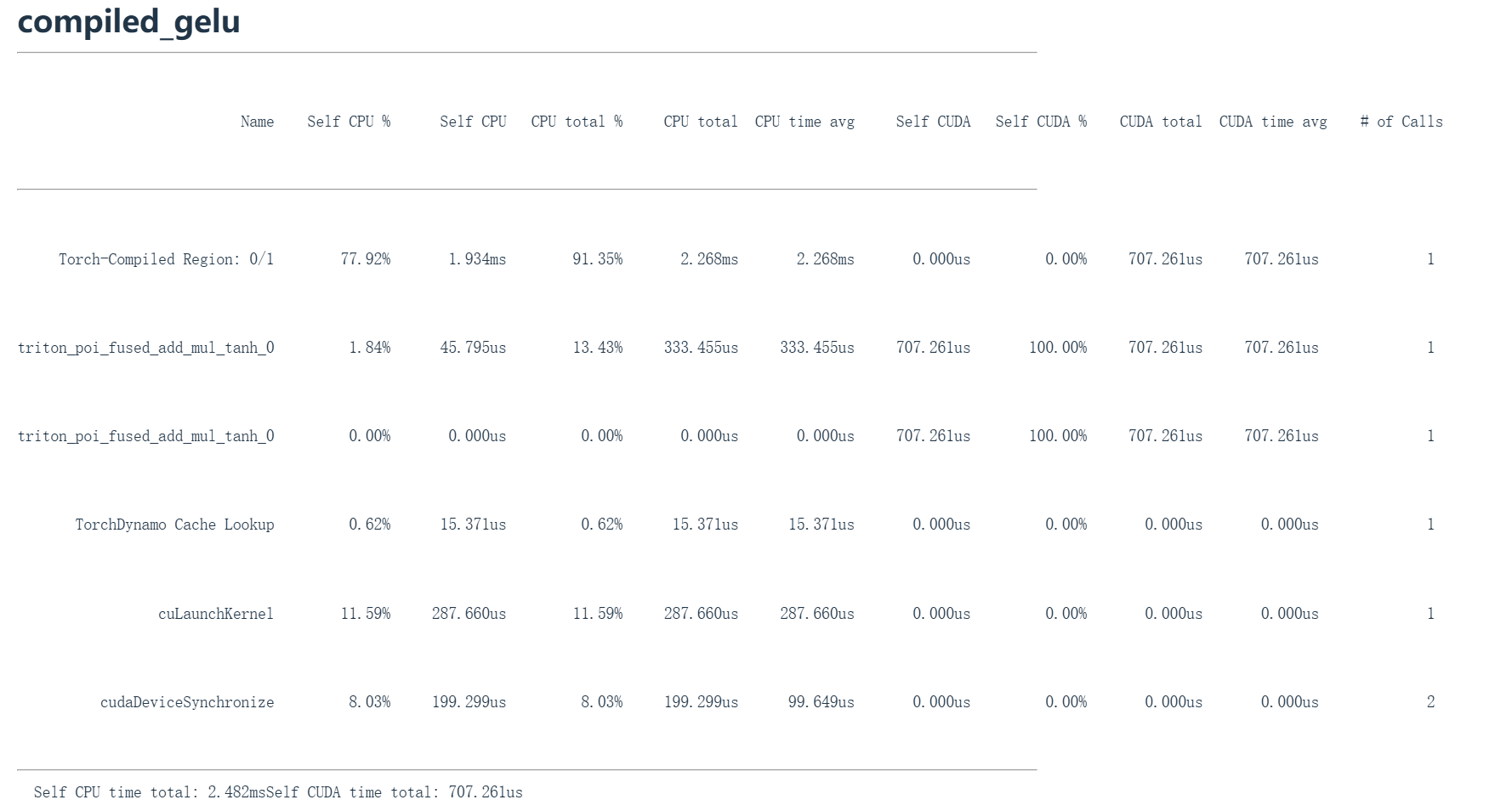
Modern JIT compilers are very powerful, capable of achieving operator fusion and other optimizations without human intervention — even slightly more optimized than what we did. So its performance is even slightly better than our code. Thus, torch.compile is truly excellent.

As for when to use torch.compile — this is a key question. For simple operations like basic operator fusion and matrix multiplication optimization, if torch.compile knows the matrix shapes, it can allocate the right kernels. In these aspects, it's already outstanding, and it's hard for humans to do better here.

But optimizations like FlashAttention 1, 2, 3 are相当 complex. Nowadays, torch.compile and Jax's XLA compiler can indeed achieve these, but that's because we only understood these were the right optimization directions after the fact. And some optimization strategies aren't easy to discover — for example, FlashAttention 3 leverages H100 hardware's底层 optimizations, which aren't intuitive for JIT compilers. These are scenarios where torch.compile struggles but humans can optimize.

However, the core point is: we shouldn't think about hand-writing CUDA kernels for every module, because that's likely a waste of time. But if you encounter complex modules when developing new architectures where GPU utilization isn't ideal but you believe there's optimization potential — that's when it's worth using Triton.