Part A: Observation Encoding

Why Compress?

Consider a 64×64 RGB game screenshot containing 64 × 64 × 3 = 12,288 pixel values. Training a policy network or dynamics model directly on these pixels introduces three problems:

1. Curse of dimensionality: High-dimensional inputs make learning extremely inefficient, requiring massive numbers of samples.
2. Redundant information: Most pixels (background, texture details) are irrelevant to decision-making.
3. Computational cost: Processing inputs with tens of thousands of dimensions at every step is prohibitively slow.

The solution is to compress the raw observation ${\mathbf{o}}_t$ (pixel image) into a low-dimensional latent vector ${\mathbf{z}}_t$ (e.g., 32 or 64 dimensions). This latent vector should retain semantic information useful for decision-making while discarding irrelevant details.

The encoder compresses the redundant high-dimensional pixel space (12,288 dimensions) into a compact, actionable latent space (32 dimensions), so that the downstream dynamics model only needs to process semantic information.

---

VAE Intuition: Learning to Compress and Reconstruct

The Variational Autoencoder (VAE)[1] is the core tool for achieving this compression. It consists of two components:

• Encoder: Maps an image $\mathbf{o}$ into latent space, outputting the mean $\mu$ (mu, the center of the distribution) and standard deviation $\sigma$ (sigma, the width of the distribution) of a distribution, then samples $\mathbf{z}$ from it.
• Decoder: Reconstructs the original image $\hat{\mathbf{o}}$ from the latent vector $\mathbf{z}$ (the hat symbol denotes "the model's estimate", distinguished from the ground-truth $\mathbf{o}$).

Key property: the latent space is continuous. This means neighboring values of $\mathbf{z}$ correspond to similar images, enabling smooth interpolation in latent space.

The VAE structure from Ha & Schmidhuber (2018): the encoder outputs mean μ and variance σ², samples z via the reparameterization trick as z = μ + σ·ε (ε ~ N(0,I)), and the decoder reconstructs the original frame from z. The reparameterization trick allows gradients to flow through the sampling operation.

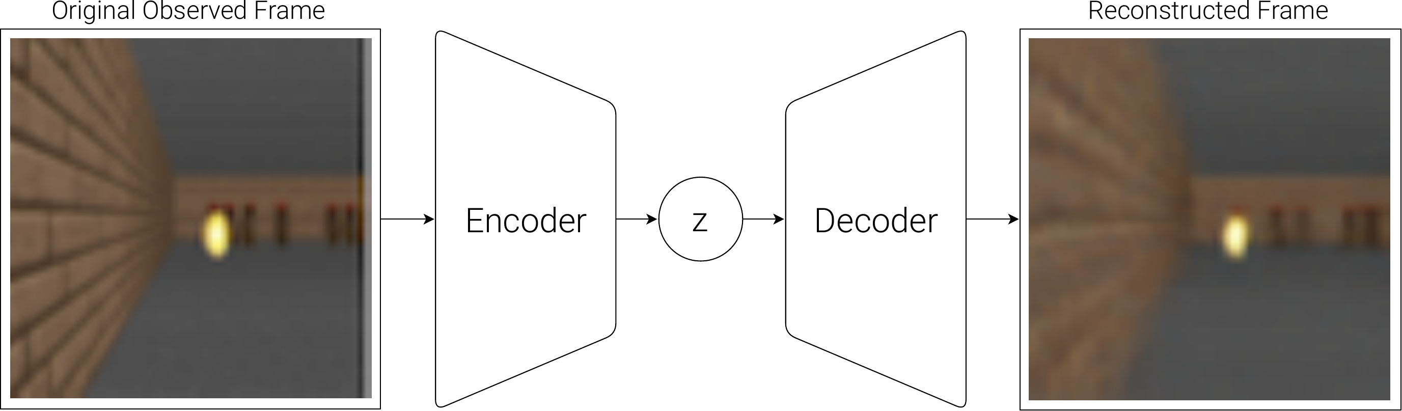
The data flows in one direction: the CNN Encoder compresses the raw image into a latent vector z, and the CNN Decoder reconstructs the image from z.

📖 Transposed Convolution (also called deconvolution): A standard convolution compresses a large feature map into a smaller one (reducing spatial resolution); a transposed convolution does the reverse, upsampling a small feature map into a larger one (increasing spatial resolution). The decoder uses transposed convolutions to progressively "restore" the low-dimensional latent vector back to the original image size.

---

ELBO Loss: Balancing Two Objectives

The training objective of a VAE is the ELBO (Evidence Lower Bound), which contains two terms:

📖 What is the ELBO? What we truly want to maximize is the probability that the model generates the real image, $\log p(\mathbf{o})$, but this quantity is intractable to compute directly (it requires integrating over all possible $\mathbf{z}$). The ELBO is a tractable lower bound on this quantity: maximizing the ELBO is equivalent to approximating this objective under a constraint. The "lower bound" in the name means exactly this: $\text{ELBO}\le \log p(\mathbf{o})$.

$${\mathcal{L}}_{\text{ELBO}}=\underset{\text{reconstruction loss}}{\underbrace{{\mathbb{E}}_{q(\mathbf{z}|\mathbf{o})}[\log p(\mathbf{o}|\mathbf{z})]}}-\underset{\text{KL divergence}}{\underbrace{D_{\text{KL}}(q(\mathbf{z}|\mathbf{o})\parallel p(\mathbf{z}))}}$$

📖 What is KL divergence? $D_{\text{KL}}(q\parallel p)$ measures the "gap" between two probability distributions: the more similar $q$ is to $p$, the closer the KL value is to 0; the larger the gap, the larger the KL value (always ≥ 0). Here it constrains the encoder's output distribution $q(\mathbf{z}|\mathbf{o})$ from straying too far from the standard normal prior $p(\mathbf{z})=\mathcal{N}(0,I)$, ensuring that different regions of the latent space can be smoothly interpolated without "holes" (regions where interpolated points decode to incoherent outputs).

Loss term	Objective	Intuition
Reconstruction loss	The decoded image should resemble the original	"Compression must still allow recovery"
KL divergence	The latent distribution should stay close to standard normal $\mathcal{N}(0,I)$	"The latent space should be well-organized and continuous"

Training maximizes the ELBO (equivalently, minimizes the negative ELBO). The two terms work together: the reconstruction loss ensures $\mathbf{z}$ retains useful information, while the KL divergence keeps the latent space structured, preventing "holes" (discontinuous regions).

📖 Reparameterization Trick: After the encoder outputs mean $\mu$ and standard deviation $\sigma$, we need to sample $\mathbf{z}$ from the distribution $\mathcal{N}(\mu ,{\sigma }^2)$. The problem with direct sampling is that the sampling operation itself is not differentiable, so gradients cannot flow from $\mathbf{z}$ back to $\mu$ and $\sigma$, preventing the encoder from being trained. The solution is to rewrite sampling as: $\mathbf{z}=\mu +\sigma \cdot \epsilon$, where $\epsilon \sim \mathcal{N}(0,I)$ is independently sampled noise (independent of the network parameters). Now $\mathbf{z}$ is differentiable with respect to $\mu$ and $\sigma$, gradients flow normally, and the encoder can be trained end-to-end.

---

CNN Encoder Structure

In practice, the encoder uses a Convolutional Neural Network (CNN) to process images, because CNNs are naturally suited for capturing local spatial features:

• Multiple convolutional layers: Each layer extracts higher-level features (edges, textures, shapes, semantics)
• Stride convolution: Progressively reduces spatial resolution, compressing information
• Fully connected layer: Flattens the final feature map and outputs two vectors, $\mu$ and $\sigma$

Typical structure: 64×64×3 → Conv(4×4, s=2) → Conv(4×4, s=2) → Conv(4×4, s=2) → Flatten → Linear → ($\mu$, $\sigma$)

---

Try It Yourself: VAE Visualization

Open demos/vae-visualizer.html in the project. You can:

1. Load a pre-trained VAE
2. Adjust individual dimensions of the latent vector $\mathbf{z}$ with sliders
3. Observe in real time how the decoder's output image changes

What to look for: some dimensions control color, some control position, some control shape. This is the disentanglement that the latent space has learned (disentanglement means that different dimensions of the latent vector each independently control one interpretable semantic factor: adjusting one dimension affects only the corresponding attribute, not the others).