1.1.1 CT (Computed Tomography)

"This is the most important advancement in the field of radiology since Röntgen's discovery of X-rays." — 1979 Nobel Prize in Physiology or Medicine Citation

🎯 An Idea That Changed the World

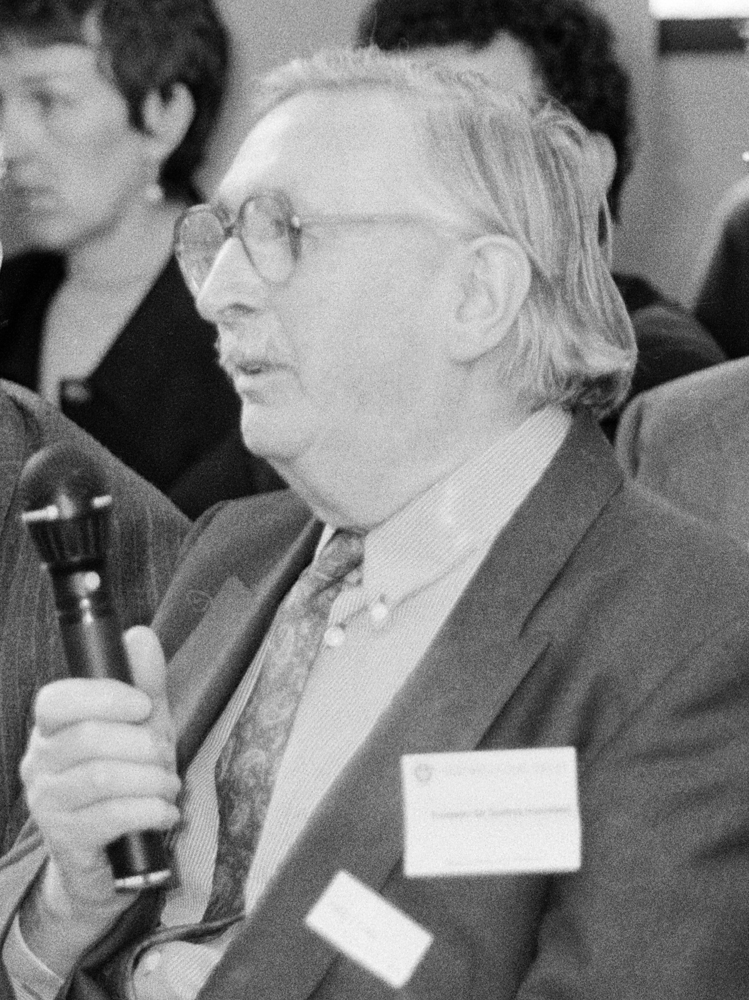Sir Godfrey Hounsfield, inventor of the CT scanner

In 1967, Godfrey Hounsfield, an engineer at EMI in the UK, was pondering a seemingly simple yet highly challenging question: Could we reconstruct the three-dimensional structure of an object by taking X-ray images from multiple angles and using a computer to process them?

The inspiration came from an everyday scenario: imagine you have a box filled with different fruits, but you can only see it from the outside. If you look from just one angle, you might only see the outermost fruits. But if you walk around the box and observe it from various angles, you can piece together the complete internal layout in your mind. Hounsfield's genius was in making the computer do this "piecing together" work.

💡 EMI and the Music Industry Connection

EMI, the company that funded Hounsfield's CT development, was one of the world's largest record companies in the 1960s (with artists including The Beatles). EMI's success in the music industry provided substantial financial resources, enabling the company to support long-term R&D projects like Hounsfield's. The CT scanner development cost approximately £100,000, a massive investment at the time.

From Concept to Reality: Five Years of Arduous Exploration

Hounsfield faced two enormous challenges:

1. Mathematical Problem: How to reconstruct the original three-dimensional image from multiple projections? Fortunately, Austrian mathematician Johann Radon had proposed the relevant mathematical theory in 1917—the Radon Transform. This theory was considered pure mathematics at the time, with no one imagining it would become the mathematical foundation of CT technology half a century later.

2. Computational Challenge: In the 1960s, computer processing power was extremely limited. The first CT scanner needed 5 minutes to acquire data, then 2.5 hours to reconstruct a single image! Today, the same task takes only a few seconds.

On October 1, 1971, the world's first clinical CT scanner was installed at Atkinson Morley Hospital in London. The first patient to undergo a CT scan was a woman suspected of having a brain tumor. When doctors saw the clearly displayed brain structures and tumor location, everyone was amazed—this was the first time in human history that the internal structure of the brain could be clearly seen without opening the skull.

🏆 Nobel Prize Glory

In 1979, Hounsfield and South African physicist Allan Cormack jointly received the Nobel Prize in Physiology or Medicine. Cormack had independently developed the mathematical theory of CT reconstruction in the 1960s, but due to lack of engineering implementation, his work was not recognized at the time. Hounsfield's engineering genius combined with Cormack's mathematical theory together ushered in the CT era.

🔬 How Does CT "See Through" the Human Body?

X-ray Attenuation: The Physical Basis of CT Imaging

When X-rays pass through the human body, they are absorbed (attenuated) to different degrees by different tissues. This attenuation follows a simplified form of the Beer-Lambert Law:

$$I=I_0\cdot e^{-\mu x}$$

Where:

• $I_0$ is the incident X-ray intensity
• $I$ is the X-ray intensity after passing through tissue
• $\mu$ is the linear attenuation coefficient of the tissue (different tissues have different values)
• $x$ is the thickness of tissue the X-ray passes through

In simple terms: X-rays are like a beam of light that gets "weakened" to different degrees when passing through different materials. Bone is dense and absorbs a lot of X-rays, so the X-rays after passing through are very weak; air hardly absorbs X-rays, so the X-ray intensity remains almost unchanged after passing through.

⚠️ Limitations of Traditional X-ray

The problem with traditional X-ray images is that they compress all depth information onto a single plane. It's like flattening a thick book and taking a photo—you can see all the text, but it's all overlapping, making it difficult to distinguish the content of each page. A small lung nodule might be obscured by ribs, and an early tumor might be lost in the overlapping images of surrounding tissues.

Tomographic Imaging: "Slicing" the Human Body Layer by Layer

CT's revolutionary breakthrough lies in tomography—instead of imaging the entire body's projection, it scans layer by layer, with each layer being a cross-section (like slicing bread).

CT's Basic Workflow:

1. Multi-angle Projection: The X-ray tube and detector rotate around the patient, taking X-ray "photographs" (projections) from hundreds of different angles
2. Measure Attenuation: Each angle measures the change in X-ray intensity after passing through the body
3. Computer Reconstruction: Using mathematical algorithms (such as filtered back-projection), reconstruct cross-sectional images from these projection data
4. 3D Imaging: Stack multiple cross-sections together to obtain three-dimensional volume data

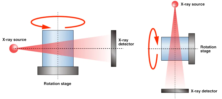CT scanning principle: X-ray source and detector rotate around the scanned object, acquiring projection data from multiple angles

💡 A Vivid Analogy

Imagine you want to guess what's inside an opaque box. If you can only shine a flashlight from one direction, the shadow information is very limited. But if you walk around the box, shining light from all 360 degrees, recording the shadow at each angle, and then using mathematical methods to "reverse engineer," you can reconstruct the three-dimensional structure inside the box. CT works exactly this way, except it uses X-rays instead of a flashlight.

Hounsfield Units (HU): The "Language" of CT

To quantify the degree of X-ray attenuation by different tissues, Hounsfield proposed a standardized scale—Hounsfield Units (HU).

Definition of HU:

$$HU=1000\times \frac{{\mu }_{tissue}-{\mu }_{water}}{{\mu }_{water}-{\mu }_{air}}$$

This formula looks complex, but it's actually quite clever:

• Water's HU value is defined as 0 (as a reference point)
• Air's HU value is defined as -1000
• Dense bone's HU value is approximately +1000

HU Value Ranges for Common Tissues:

Tissue Type	HU Range	Clinical Significance
Air	-1000	Lungs, airways
Fat	-120 ~ -90	Subcutaneous fat, abdominal fat
Water	0	Reference standard
Blood	+30 ~ +45	Vessels, hemorrhage
Muscle	+10 ~ +40	Soft tissue
Gray Matter	+37 ~ +45	Brain tissue
White Matter	+20 ~ +30	Brain tissue
Liver	+40 ~ +60	Parenchymal organs
Bone	+700 ~ +3000	Bone density assessment
Metal Implants	> +3000	Causes artifacts

🎨 Window Width and Level: CT Image "Palette"

Since the human eye can only distinguish about 20-30 gray levels, while CT's HU value range spans from -1000 to +3000, we need to select a "window" to display tissues of interest. For example:

• Lung Window (width 1500, level -600): Suitable for observing lung structures
• Mediastinal Window (width 350, level 50): Suitable for observing heart, vessels
• Bone Window (width 2000, level 300): Suitable for observing bones This is like using different "filters" to highlight different tissue structures.

📈 Evolution of CT Technology: From 5 Minutes to Sub-second

Since its birth in 1971, CT technology has undergone multiple revolutionary upgrades. Each generation of CT advancement has greatly expanded clinical applications and improved diagnostic capabilities.

First Generation CT (1971-1975): Translate-Rotate

Technical Features:

• Single Detector: Only one X-ray tube and one detector
• Scanning Method: X-ray tube and detector translate together to scan a line, then rotate 1 degree, then translate to scan the next line
• Scan Time: 5-7 minutes/slice (180 translations × 180 angles)
• Image Matrix: 80×80 pixels

Clinical Applications:

• Limited to head scanning only (because patients needed to remain still for a long time)
• Mainly used for diagnosing brain tumors and cerebral hemorrhage

⏱️ The Long Wait

Imagine a patient needing to remain completely still on the scanning bed for over 5 minutes—any slight movement would blur the image. This was nearly impossible for emergency patients or children.

Second Generation CT (1975-1980): Fan-Beam Scanning

Technical Improvements:

• Multiple Detector Array: 3-30 detectors arranged in a row
• Fan-Beam X-rays: X-ray beam in fan shape, can simultaneously illuminate multiple detectors
• Scan Time: 20-60 seconds/slice (dramatically shortened!)

Clinical Significance:

• Shortened scan time made body scanning possible
• Patient comfort greatly improved

Third Generation CT (1980-1990): Rotate-Rotate

Technical Breakthrough:

• Large Detector Array: Hundreds of detectors arranged in an arc
• Synchronous Rotation: X-ray tube and detector array rotate together around the patient
• Scan Time: 2-10 seconds/slice
• Image Quality: Resolution improved to 512×512 pixels

Expanded Clinical Applications:

• Chest, abdomen, and pelvis scans became routine examinations
• Dynamic contrast-enhanced scanning became possible (continuous scanning after contrast injection)

🚀 Speed Leap

From first generation's 5 minutes to third generation's few seconds, scanning speed increased nearly 100-fold! This transformed CT from "laboratory equipment" to truly "routine clinical tool."

Fourth Generation CT (1980s): Fixed Detector Ring

Design Philosophy:

• Fixed Detector Ring: Complete 360-degree detector ring remains stationary
• Rotating X-ray Tube: Only the X-ray tube rotates around the patient
• Advantage: Theoretically could reduce ring artifacts

Reality:

• Due to high cost and complex maintenance, fourth generation CT did not become mainstream
• Third generation CT solved ring artifact problems through algorithmic improvements and ultimately dominated the market

Helical CT / Slip-Ring CT (1990s): The Revolution of Continuous Scanning

Revolutionary Innovation:

• Slip-Ring Technology: X-ray tube and detector can rotate continuously (no need to return)
• Continuous Scanning: Patient bed moves continuously, X-ray tube rotates continuously, scanning trajectory is helical
• 3D Imaging: Can obtain true three-dimensional volume data, not layer-by-layer 2D slices

Clinical Significance:

• Dramatically Shortened Scan Time: Entire chest or abdomen in just 20-30 seconds
• Reduced Respiratory Artifacts: Patient only needs to hold breath once
• 3D Reconstruction: Can perform multiplanar reconstruction (MPR), maximum intensity projection (MIP), volume rendering (VR)

Helical CT scanning trajectory diagram: X-ray source rotates continuously while patient bed moves simultaneously, forming a helical scanning path

🌀 Why Called "Helical" CT?

Imagine the X-ray tube rotating around the patient while the patient bed moves at constant speed. From the X-ray tube's perspective, its motion trajectory looks like a helix (or spring). This is the origin of the name "Helical CT" (or Spiral CT).

Multi-Slice CT (MSCT, 2000s): Dual Enhancement of Speed and Resolution

Technical Progress:

• Multi-Row Detectors: Evolved from single-row to 4-slice, 16-slice, 64-slice, 128-slice, 320-slice
• Faster Scanning Speed: 320-slice CT can complete entire heart scan within one heartbeat
• Higher Resolution: Sub-millimeter spatial resolution

MSCT Generation Milestones:

Year	Slices	Scan Time (Full Chest)	Clinical Breakthrough
1998	4-slice	~20 seconds	Cardiac imaging initially feasible
2002	16-slice	~10 seconds	Coronary artery imaging
2004	64-slice	~5 seconds	Cardiac imaging becomes routine
2007	128-slice	~3 seconds	Whole-body trauma scanning
2007	320-slice	<1 second	Single heartbeat cardiac imaging

💓 Challenge of Cardiac Imaging

The heart is a constantly beating organ, making it difficult for traditional CT to obtain clear cardiac images. 64-slice and higher MSCT have sufficiently high temporal resolution (~100ms) to complete scanning during the brief "stationary" moment of cardiac diastole, thus obtaining clear coronary artery images. This made CT coronary angiography (CTCA) a non-invasive cardiac examination method.

Dual-Source CT and Dual-Energy CT (2010s): From Structure to Function

Dual-Source CT (DSCT):

• Two Sets of X-ray Tube and Detector Systems: Installed at 90-degree angle on the same gantry
• Ultra-High Temporal Resolution: ~75ms (twice that of single-source CT)
• Clinical Advantages:
  • Further improved cardiac imaging quality, no need for beta-blockers to lower heart rate
  • Suitable for patients with arrhythmia

Dual-Energy CT (DECT):

• Two Different Energy X-rays: Low energy (80kV) and high energy (140kV)
• Material Separation Capability: Different materials have different attenuation characteristics for different energy X-rays
• Clinical Applications:
  • Differentiation of Uric Acid and Non-Uric Acid Stones: A powerful tool for gout diagnosis
  • Quantitative Analysis of Iodine Contrast: Assess tumor blood supply
  • Virtual Non-Contrast: "Subtract" iodine contrast from enhanced scan, reducing radiation dose
  • Virtual Monoenergetic Images: Reduce metal artifacts and beam hardening artifacts

🎨 The "Magic" of Dual-Energy CT

Imagine you have two photos, one taken with red light and one with blue light. Some objects are bright in red light but dark in blue light; while other objects are the opposite. By comparing these two photos, you can distinguish different objects. Dual-energy CT uses this principle, comparing the attenuation differences of low-energy and high-energy X-rays to distinguish different materials (such as iodine, calcium, uric acid, etc.).

Photon-Counting CT (2020s): Next-Generation CT Technology

Technological Innovation:

• Photon-Counting Detector: Directly counts each X-ray photon, rather than measuring total energy
• Energy Resolution Capability: Can simultaneously obtain images at multiple energy levels (not just two)
• Advantages:
  • Higher Spatial Resolution: Up to 0.2mm (traditional CT ~0.5mm)
  • Lower Radiation Dose: 40-50% reduction
  • Better Contrast Resolution: Clearer soft tissue details
  • Eliminates Electronic Noise: Higher image quality

Clinical Prospects:

• In 2021, Siemens launched the first clinical photon-counting CT (NAEOTOM Alpha)
• Expected to become the mainstream direction of CT technology for the next 10-20 years

🔬 From "Analog" to "Digital"

Traditional CT detectors are like a bucket, measuring "how much water was collected" (total energy). Photon-counting detectors are like a precision counter, able to count "how many drops of water fell" (photon count), and can also distinguish the "size" of each drop (energy). This transition from "analog" to "digital" brings a qualitative leap.

📊 Overview of CT Technology Evolution

Let's summarize 50 years of CT technology evolution in a table:

Generation	Era	Scanning Method	Scan Time	Spatial Resolution	Key Breakthrough	Clinical Significance
1st Gen	1971-1975	Translate-Rotate	5-7 min/slice	3mm	First tomographic imaging	Brain imaging
2nd Gen	1975-1980	Fan-beam	20-60 sec/slice	1.5mm	Multiple detectors	Body scanning feasible
3rd Gen	1980-1990	Rotate-Rotate	2-10 sec/slice	1mm	Large detector array	Became routine exam
4th Gen	1980s	Fixed detector ring	2-10 sec/slice	1mm	Fixed detectors	Not mainstream
Helical CT	1990s	Continuous rotation	20-30 sec/organ	1mm	3D imaging	3D reconstruction
4-16 Slice	1998-2002	Multi-slice helical	10-20 sec/organ	0.6mm	Multi-row detectors	Initial cardiac imaging
64-Slice	2004-2010	Multi-slice helical	5-10 sec/organ	0.5mm	High temporal resolution	Routine coronary imaging
128-320 Slice	2007-2015	Multi-slice helical	<5 sec/organ	0.5mm	Ultra-fast scanning	Single heartbeat imaging
Dual-Source/Energy	2006-present	Dual-source system	<5 sec/organ	0.5mm	Functional imaging	Material separation
Photon-Counting	2021-future	Photon-counting	<5 sec/organ	0.2mm	Energy resolution	Ultra-high resolution

🎯 Clinical Significance of CT Technology Evolution

Each advancement in CT technology has greatly expanded clinical diagnostic capabilities:

Evolution Dimension	Early CT (1970-1990s)	Modern CT (2000s-present)	Clinical Significance
Image Quality	Can see brain tumor existence	Can see smaller lesions, distinguish tissue composition	From "visible" to "clear," early diagnosis capability greatly improved
Scan Objects	Can only scan stationary organs (brain, liver)	Can scan rapidly moving organs (heart, arrhythmia)	From "static organs" to "dynamic organs," cardiac imaging became possible
Diagnostic Capability	Can only see anatomical structure ("what it looks like")	Can assess function and metabolism ("how it functions," "what composition")	From "morphological diagnosis" to "functional diagnosis," providing more comprehensive information
Radiation Dose	Higher radiation dose, limiting application scope	50-70% reduction through iterative reconstruction and photon-counting technology	From "high radiation" to "low dose," making CT screening possible

☢️ Radiation Dose Considerations

Although CT radiation dose has been greatly reduced, it still requires careful use. A chest CT scan has a radiation dose of about 7mSv, equivalent to 2-3 years of natural background radiation. Therefore, CT examinations should follow the "ALARA principle" (As Low As Reasonably Achievable), minimizing radiation dose while ensuring diagnostic quality.

🔑 Key Takeaways

1. Essence of CT: Through multi-angle X-ray projections, using computers to reconstruct cross-sectional images of the human body, achieving "layer-by-layer viewing" tomographic imaging.

2. Hounsfield Units: The "language" of CT images, with water at 0, air at -1000, bone at +1000, and different tissues having different HU value ranges.

3. Technology Evolution: From first generation's 5 minutes/slice to modern sub-second full-organ scanning, CT technology has undergone 50 years of continuous progress.

4. Expanded Clinical Applications: From initial brain imaging to whole-body organ imaging, then to cardiac imaging and functional imaging, CT's application scope continues to expand.

5. Future Direction: Photon-counting CT represents next-generation technology, bringing higher resolution, lower radiation dose, and stronger material separation capabilities.

---

💡 Next Steps

Now you understand the basic principles and technological evolution of CT. In Chapter 3, we will delve into the mathematical principles of CT image reconstruction, including Radon transform, filtered back-projection algorithms, and other core technologies. In Chapter 2, we will learn CT raw data preprocessing methods, including beam hardening correction, metal artifact suppression, and other practical techniques.