5.2 Segmentation: U-Net and its variants

This mainline page answers the Chapter 5 question "Why does segmentation work?" Full runnable scripts, demo outputs, and environment notes are collected in 5.6 Code Labs / Practice Appendix and src/ch05/README_EN.md.

"U-Net is not just a network architecture, but a revolutionary thinking in medical image segmentation—proving that carefully designed architectures can surpass brute-force training on large datasets." — — Ronneberger et al., "U-Net: Convolutional Networks for Biomedical Image Segmentation", MICCAI 2015

Readers often feel classification is not enough in cases such as:

• measuring tumor volume;
• outlining the lung field precisely;
• defining where a radiotherapy target should stop slice by slice;
• describing the spatial relation between lesions and nearby anatomy.

⚡ U-Net's Success in Medical Imaging

Special Challenges of Medical Image Segmentation

Compared to natural image segmentation, medical image segmentation faces unique challenges:

Challenge	Natural Image Segmentation	Medical Image Segmentation	U-Net's Solution
Data Scarcity	Millions of labeled images	Usually only hundreds	Skip connections enhance feature transfer
Boundary Precision Requirements	Relatively relaxed	Sub-pixel level precision requirements	Multi-scale feature fusion
Class Imbalance	Relatively balanced	Lesion regions usually very small	Deep supervision techniques
3D Structure Understanding	Primarily 2D	Need 3D context information	Extended to 3D versions

U-Net's Revolutionary Design Philosophy

U-Net's success stems from three core design principles:

1. Encoder-Decoder Structure: Compress information like a funnel, then gradually restore
2. Skip Connections: Directly transfer shallow features to avoid information loss
3. Fully Convolutional Network: Adapt to input images of any size

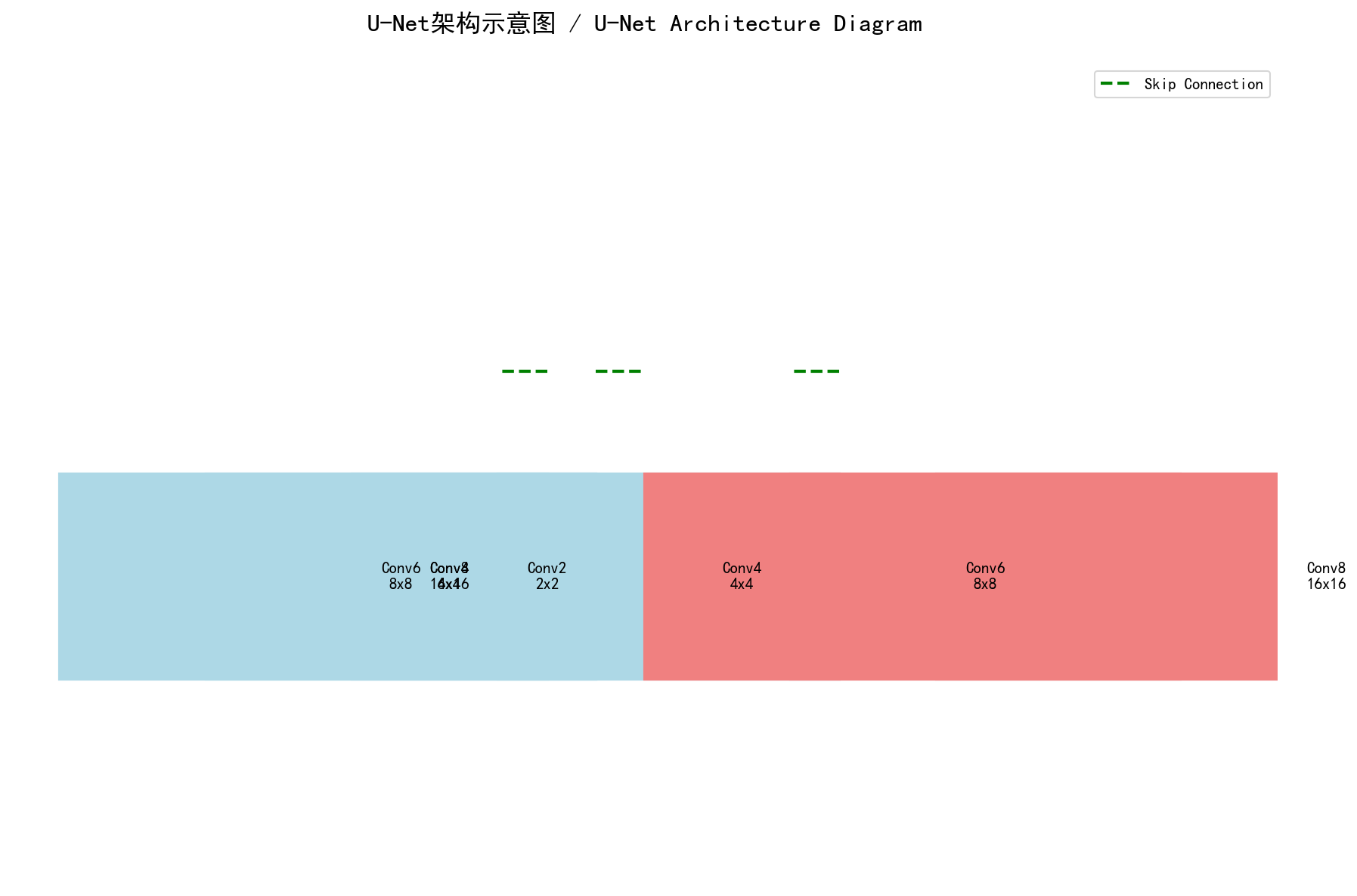U-Net's core idea: Encoder extracts semantic features, decoder restores spatial resolution, skip connections ensure details aren't lost - Custom diagram

Intuitive explanation

Before thinking of segmentation as a complicated network, it is better to think of it as: turning image reading into measurable regions.

Classification answers whether something is present. Segmentation goes further and answers:

• where the region is;
• how large it is;
• what the volume is;
• how its boundary relates to nearby structures.

U-Net became classic not because it is simply deep, but because it captures one core tension:

• deep features are better at saying what something is;
• shallow features are better at preserving where it is.

So the network extracts semantics on the way down and reconnects spatial detail on the way back up.

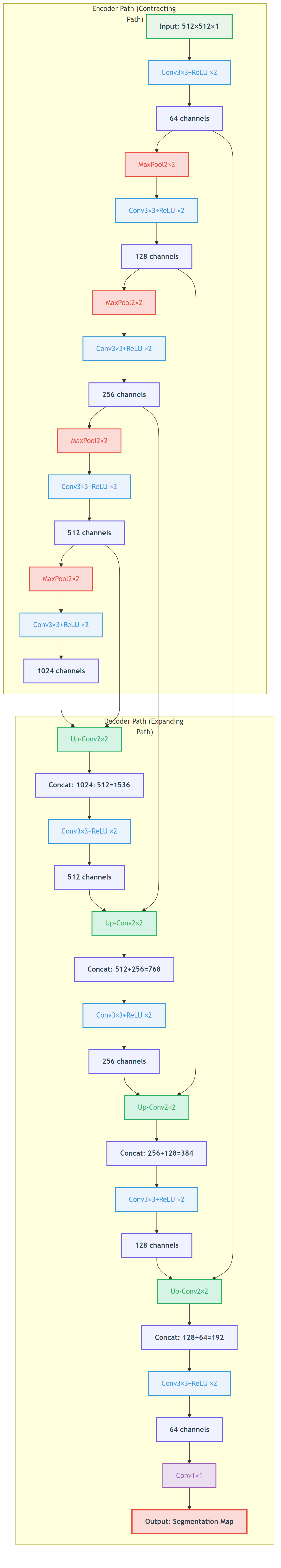Figure: the key to U-Net is not just downsampling and upsampling, but the skip connections that bring boundary detail back.

Core method

This section keeps only 4 key ideas.

1. Be clear about the output

Segmentation usually outputs not a single score, but a probability map or mask at the same scale as the input, or one that can be mapped back to the original image.

2. Preserve semantics and boundaries together

The encoder extracts high-level semantics; the decoder restores spatial resolution; skip connections prevent small structures and boundaries from disappearing completely during downsampling.

3. Keep labels perfectly aligned with images

In segmentation, one of the biggest failure modes is not weak augmentation but desynchronized transforms between image and mask. Once they drift apart, the model is no longer learning true boundaries.

4. Do not judge quality by loss alone

Dice, IoU, sensitivity, connected-component behavior, and post-processing results often say more about practical segmentation quality than training loss by itself.

Typical case

Case 1: Lung field segmentation

• Goal: obtain a lung mask from chest CT.
• Value: provides an ROI for later nodule detection, infection analysis, and quantitative measurement.
• Local code: src/ch05/lung_segmentation_network/main.py.

Case 2: Organ or tumor segmentation

• Goal: precise contours for liver, pancreas, brain tumor, prostate, and similar targets.
• Value: volume estimation, disease burden tracking, and radiotherapy target delineation.
• Extensions: 2D U-Net, 3D U-Net, Attention U-Net, nnU-Net.

Case 3: Augmentation in segmentation tasks

• Goal: make image and mask undergo the same geometric transform.
• Local code: src/ch05/medical_segmentation_augmentation/main.py.
• Reminder: when the image changes, the label must change in sync.

Practice tips

The main text only keeps short code fragments for intuition; full training, evaluation, and visualization live in src/ch05/.

1. A minimal convolution block

class MultisequenceSegmentationUNet(nn.Module):
    def __init__(self, num_sequences=4, num_classes=4):
        super().__init__()

        # Create independent encoders for each sequence
        self.sequence_encoders = nn.ModuleList([
            self.create_encoder(1, 64) for _ in range(num_sequences)
        ])

        # Feature fusion module
        self.feature_fusion = nn.Conv2d(64 * num_sequences, 64, 1)

        # Shared decoder
        self.decoder = self.create_decoder(64, num_classes)

    def forward(self, sequences):
        # Independent encoding for each sequence
        encoded_features = []
        for seq, encoder in zip(sequences, self.sequence_encoders):
            encoded, skip = encoder(seq)
            encoded_features.append(encoded)

        # Feature fusion
        fused_features = torch.cat(encoded_features, dim=1)
        fused_features = self.feature_fusion(fused_features)

        # Decode
        return self.decoder(fused_features)

Specialized Strategies for X-ray Image Segmentation

Anatomical Prior Constraints

class AnatomicallyConstrainedUNet(nn.Module):
    def __init__(self, base_unet):
        super().__init__()
        self.base_unet = base_unet
        self.anatomy_prior = AnatomicalPriorNet()  # Anatomical prior network

    def forward(self, x):
        # Base segmentation result
        segmentation = self.base_unet(x)

        # Anatomical prior
        anatomy_constraint = self.anatomy_prior(x)

        # Constrained fusion
        constrained_segmentation = segmentation * anatomy_constraint

        return constrained_segmentation

💡 Training Tips & Best Practices

Medical-Specific Data Augmentation Strategies

Medical image segmentation requires special consideration of anatomical and clinical constraints. Unlike natural image segmentation, medical augmentation must maintain anatomical reasonableness and clinical relevance.

Recommended Medical Augmentation Techniques

• Elastic Deformation: Simulate physiological motion (respiratory, cardiac movement) with non-rigid grid deformation
• Intensity Transformation: Simulate variation in different scanning parameters and protocols across institutions
• Noise Addition: Model real clinical environment noise to improve robustness to low-quality images from mobile devices or emergency scenarios
• Partial Occlusion: Simulate metal artifacts from implants or motion artifacts from patient movement

Augmentation Methods to Avoid

• Random Rotation: May destroy anatomical structure that should maintain fixed orientations
• Extreme Scaling: May introduce unrealistic deformations inconsistent with physiological changes
• Color/Hue Transformation: Medical images are typically grayscale with specific physical meanings (HU values, T1/T2 weightings)

Clinical Principle: All augmentation strategies must undergo physician verification to ensure they create clinically realistic variations rather than introducing medical artifacts.

Data Augmentation Strategies

Special data augmentation for medical image segmentation:

def medical_segmentation_augmentation(image, mask):
    """
    Special data augmentation for medical image segmentation
    """
    # 1. Elastic deformation (maintain anatomical reasonableness)
    if np.random.rand() < 0.5:
        image, mask = elastic_deformation(image, mask)

    # 2. Rotation (multiples of 90 degrees)
    if np.random.rand() < 0.3:
        angle = np.random.choice([90, 180, 270])
        image = rotate(image, angle)
        mask = rotate(mask, angle)

    # 3. Flip (left-right symmetry)
    if np.random.rand() < 0.5:
        image = np.fliplr(image)
        mask = np.fliplr(mask)

    # 4. Intensity transformation
    if np.random.rand() < 0.3:
        image = intensity_transform(image)

    return image, mask

📖 Complete Code Example: medical_segmentation_augmentation/ - Complete medical image segmentation augmentation implementation with multiple augmentation strategies and clinical validation

Medical Image Segmentation Augmentation Demonstration

Practical Enhancement Effect Display

To understand the impact of different augmentation techniques on medical image segmentation, we create a simulated CT lung image and demonstrate how four medical-specific augmentation techniques affect the image while maintaining clinical validity.

Medical Segmentation Augmentation Demo

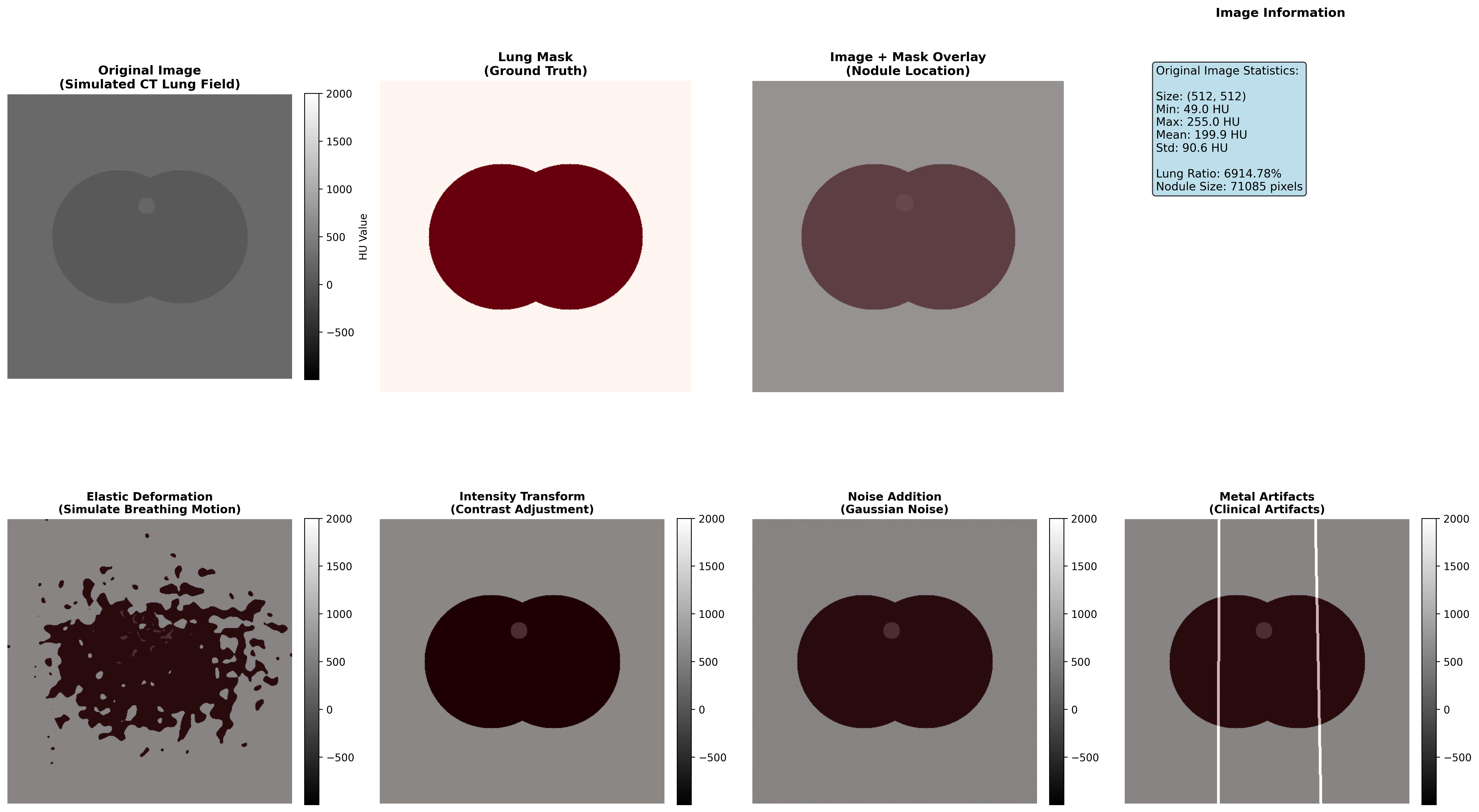
Demonstration of four medical-specific augmentation techniques: elastic deformation simulates respiratory motion, intensity transformation adapts to different scanning protocols, noise addition models real clinical environment, and metal artifacts simulate implant influences

Augmentation Technique Effectiveness Analysis

Enhancement Type	Technical Principle	Clinical Significance	Application Scenarios	Implementation Caution
Elastic Deformation	Non-rigid grid deformation with interpolation	Simulate respiratory motion, cardiac pulsation	Thoracic and abdominal organs	Deformation intensity must remain within physiological range
Intensity Transformation	Contrast and brightness adjustment	Adapt to different scanning protocols, multi-center data unification	Multi-institution data fusion, cross-protocol analysis	Must preserve HU value medical meaning and tissue contrast relationships
Noise Addition	Gaussian or Poisson noise injection	Improve model robustness to low-quality images	Mobile devices, emergency scenarios, portable ultrasound	Noise characteristics should match actual device specifications
Metal Artifacts	Linear high-density streak simulation	Simulate metal implant influences (dental fillings, hip prostheses, pacemakers)	Orthopedic and dental imaging, cardiac device patients	Artifact morphology should match actual implant types

Execution Results Analysis

Medical Image Segmentation Augmentation Analysis Report


def double_conv(in_channels, out_channels):
    return nn.Sequential(
        nn.Conv2d(in_channels, out_channels, 3, padding=1),
        nn.ReLU(inplace=True),
        nn.Conv2d(out_channels, out_channels, 3, padding=1),
        nn.ReLU(inplace=True),
    )

2. The key skip-connection action: concatenation

import pydensecrf.densecrf as dcrf

class CRFPostProcessor:
    def __init__(self, num_iterations=5):
        self.num_iterations = num_iterations

    def __call__(self, image, unary_probs):
        """
        CRF post-processing: consider inter-pixel relationships
        """
        h, w = image.shape[:2]

        # Create CRF model
        d = dcrf.DenseCRF2D(w, h, num_classes=unary_probs.shape[0])

        # Set unary potentials
        U = unary_probs.reshape((unary_probs.shape[0], -1))
        d.setUnaryEnergy(U)

        # Set binary potentials (inter-pixel relationships)
        d.addPairwiseGaussian(sxy=3, compat=3)
        d.addPairwiseBilateral(sxy=80, srgb=13, rgbim=image, compat=10)

        # Inference
        Q = d.inference(self.num_iterations)

        return np.array(Q).reshape((unary_probs.shape[0], h, w))

📈 Performance Evaluation & Model Comparison

Clinical Significance of Performance Metrics

Segmentation quality metrics have direct clinical implications:

Metric	Clinical Application	Excellent Standard	Good Standard	Improvement Strategy
Dice Coefficient	Lesion volume assessment for treatment planning	>0.85	>0.75	Improve boundary accuracy through loss function refinement
Intersection over Union (IoU)	Overlap region calculation for surgical planning	>0.80	>0.70	Enhance overall consistency through architecture optimization
Sensitivity (Recall)	False negative control - avoiding missed lesions	>0.95	>0.90	Reduce false negatives through weighted loss or class rebalancing
Specificity	False positive control - avoiding over-segmentation	>0.90	>0.85	Reduce false positives through stronger anatomical constraints
Hausdorff Distance	Boundary deviation measurement for surgical navigation	<5 mm	<10 mm	Refine boundary precision through boundary-aware losses

Clinical Decision Guidelines:

• For surgical planning: Require Dice >0.85 and Hausdorff <5mm
• For volume assessment: Require Dice >0.80 and IoU >0.75
• For lesion detection: Require Sensitivity >0.95 to minimize false negatives

Common Training Issues and Diagnostic Solutions

Issue 1: Model Over-predicts Background

Symptoms: Low Dice coefficient, high specificity Root Cause: Class imbalance in training data, excessive learning rate, insufficient data augmentation Solution Strategy:

• Adjust loss function weights: Increase lesion class weight by 2-5×
• Reduce learning rate by 50% and train longer
• Add aggressive data augmentation for minority class

Issue 2: Blurry Segmentation Boundaries

Symptoms: Low boundary Dice coefficient despite acceptable overall Dice Root Cause: Loss of fine spatial information in skip connections, insufficient decoder resolution Solution Strategy:

• Add explicit boundary loss term: loss_total = loss_main + 0.3 × loss_boundary
• Verify skip connection alignment between encoder and decoder
• Increase decoder intermediate channels

Issue 3: Complete Miss of Small Targets

Symptoms: Good performance on large lesions, completely missing small targets Root Cause: Large receptive field of deep layers, insufficient multi-scale information Solution Strategy:

• Implement multi-scale training: Train on multiple image resolutions
• Add dedicated small lesion branch in decoder
• Apply progressive training: Start with large targets, add small targets later

Evaluation Metrics

1. Dice Coefficient

$$\text{Dice}=\frac{2|P\cap G|}{|P|+|G|}$$

Where:

• $P$: Predicted segmentation result
• $G$: Ground truth annotation

2. Intersection over Union (IoU)

$$\text{IoU}=\frac{|P\cap G|}{|P\cup G|}$$

3. Hausdorff Distance

Hausdorff distance measures the maximum deviation of segmentation boundaries:

$$H(A,B)=max\{h(A,B),h(B,A)\}$$

Where:

$$h(A,B)=\underset{a\in A}{max}\underset{b\in B}{min}||a-b||$$

Performance Comparison of Different U-Net Variants

Model	Dice Score	Parameter Count	Training Time	Applicable Scenarios
Original U-Net	0.85-0.90	~31M	Moderate	2D image segmentation
V-Net	0.88-0.93	~48M	Longer	3D volume data
U-Net++	0.87-0.92	~42M	Longer	Fine boundary requirements
Attention U-Net	0.89-0.94	~35M	Moderate	Large background noise
nnU-Net	0.91-0.96	Variable	Auto-optimized	General scenarios

🏥 Clinical Application Case Studies

Case 1: Brain Tumor Segmentation

Task Description

Use multi-sequence MRI to segment different brain tumor regions:

• Necrotic core
• Edema region
• Enhancing tumor

Data Characteristics

• Multi-modal input: T1, T1ce, T2, FLAIR
• 3D volume data
• Extremely imbalanced classes

U-Net Architecture Adaptation

class BrainTumorSegmentationNet(nn.Module):
    def __init__(self):
        super().__init__()

        # Multi-sequence encoders
        self.t1_encoder = EncoderBlock(1, 64)
        self.t1ce_encoder = EncoderBlock(1, 64)
        self.t2_encoder = EncoderBlock(1, 64)
        self.flair_encoder = EncoderBlock(1, 64)

        # Feature fusion
        self.fusion_conv = nn.Conv2d(256, 64, 1)

        # Decoder (4-class segmentation: background + 3 tumor classes)
        self.decoder = UNetDecoder(64, 4)

    def forward(self, t1, t1ce, t2, flair):
        # Encode each sequence
        _, t1_features = self.t1_encoder(t1)
        _, t1ce_features = self.t1ce_encoder(t1ce)
        _, t2_features = self.t2_encoder(t2)
        _, flair_features = self.flair_encoder(flair)


def fuse_skip(upsampled, shallow_feature):
    return torch.cat([upsampled, shallow_feature], dim=1)

3. A minimal Dice implementation

import torch


def dice_score(pred_mask, true_mask, eps=1e-6):
    inter = (pred_mask * true_mask).sum()
    union = pred_mask.sum() + true_mask.sum()
    return (2 * inter + eps) / (union + eps)

🎯 Core Insights & Future Outlook

1. U-Net's Core Advantages:

   • Skip connections solve deep learning feature loss problems
   • Encoder-decoder structure balances semantic information and spatial precision
   • End-to-end training simplifies the segmentation pipeline

2. Importance of Modality Adaptation:

   • CT: Utilize HU value prior knowledge
   • MRI: Multi-sequence information fusion
   • X-ray: Anatomical prior constraints

3. Loss Function Design:

   • Dice Loss addresses class imbalance
   • Focal Loss focuses on hard samples
   • Combined loss functions improve performance

4. Practical Tips:

   • Data augmentation maintains anatomical reasonableness
   • Multi-metric training process monitoring
   • Post-processing improves final accuracy

5. Future Development Directions:

   • Transformer-based segmentation models
   • Self-supervised learning to reduce annotation dependency
   • Cross-modal domain adaptation

🔗 Typical Medical Datasets and Paper URLs Related to This Chapter

Details

Datasets

Dataset	Purpose	Official URL	License	Notes
BraTS	Brain Tumor Multi-sequence MRI Segmentation	https://www.med.upenn.edu/cbica/brats/	Academic use free	Most authoritative brain tumor dataset
LUNA16	Lung Nodule Detection and Segmentation	https://luna16.grand-challenge.org/	Public	Standard lung nodule dataset
MSD	Multi-organ Segmentation	https://medicaldecathlon.grand-challenge.org/	Public	Multi-organ segmentation challenge
ATLAS	Cardiac CT/MRI Segmentation	http://medicaldecathlon.grand-challenge.org/	Academic use free	Cardiac segmentation dataset
KiTS21	Kidney Tumor Segmentation	https://kits21.kits-challenge.org/	Public	Kidney tumor segmentation
ISBI	Cell Segmentation	http://brainiac2.mit.edu/isbi/	Public	Electron microscope cell segmentation

Papers

Paper Title	Keywords	Source	Notes
U-Net: Convolutional Networks for Biomedical Image Segmentation	U-Net segmentation network	arXiv:1505.04597	Original U-Net paper, pioneering encoder-decoder architecture for medical image segmentation
U-Net++: A Nested U-Net Architecture for Medical Image Segmentation	Deep supervision segmentation	arXiv:1807.10165	U-Net++ improvement, enhancing segmentation accuracy through deep supervision and dense connections
nnU-Net: A Framework for Automatic, Deep Learning-Based Biomedical Image Segmentation	Automatic segmentation framework	Nat Methods 18, 203–211 (2021)	nnU-Net automation framework, achieving SOTA performance in multiple medical segmentation tasks
V-Net: Fully Convolutional Neural Networks for Volumetric Medical Image Segmentation	3D medical segmentation	2016 Fourth International Conference on 3D Vision	V-Net, fully convolutional network designed specifically for 3D medical image segmentation
Attention U-Net: Learning Where to Look for a Pancreas	Attention mechanism segmentation	arXiv	Introducing attention mechanism in medical segmentation to improve target region recognition
Deep Learning for Brain Tumor Segmentation: A Survey	Brain tumor segmentation review	Springer Journal: Complex & Intelligent Systems	Comprehensive review of deep learning methods and comparisons for brain tumor segmentation
3D U-Net: Learning Dense Volumetric Segmentation from Sparse Annotation	3D sparse segmentation	arXiv:1606.06650	3D U-Net extension, suitable for sparsely annotated 3D medical image segmentation

Open Source Libraries

Library	Function	GitHub/Website	Purpose
TorchIO	Medical Image Transformation Library	https://torchio.readthedocs.io/	Medical image data augmentation
nnU-Net	Automatic Segmentation Framework	https://github.com/MIC-DKFZ/nnunet	Medical image segmentation framework
MONAI	Deep Learning Medical AI	https://monai.io/	Medical imaging deep learning
SimpleITK	Medical Image Processing	https://www.simpleitk.org/	Image processing toolkit
ANTsPy	Image Registration and Analysis	https://github.com/ANTsX/ANTsPy	Advanced image analysis
medpy	Medical Image Processing	https://github.com/loli/medpy	Medical imaging algorithm library
DeepLabv3+	Semantic Segmentation	https://github.com/tensorflow/models/tree/master/research/deeplab	DeepLabv3+ implementation

The next section moves to classification and detection because not every workflow needs a fine contour first. Many clinical pipelines start by asking: is there disease, what is it, and roughly where should we look?