1.1.2 MRI (Magnetic Resonance Imaging)
"If CT allows us to see the anatomical structure of the human body, then MRI allows us to see the intrinsic properties of tissues."
🎯 A Wonderful Journey from Physics Laboratory to Clinical Diagnosis
Discovery of Nuclear Magnetic Resonance
In 1946, two physicists almost simultaneously and independently discovered a wonderful phenomenon: Nuclear Magnetic Resonance (NMR).
- Felix Bloch (Stanford University): Observed nuclear magnetic resonance in solids
- Edward Purcell (Harvard University): Observed nuclear magnetic resonance in liquids
These two scientists jointly received the 1952 Nobel Prize in Physics. But at the time, this was purely a physics discovery, mainly used to study the molecular structure of matter, with no one imagining it would completely transform medical diagnosis.
💡 Why Called "Nuclear" Magnetic Resonance?
"Nuclear" refers to atomic nuclei (mainly hydrogen nuclei, i.e., protons). However, because the word "nuclear" easily evokes associations with nuclear radiation, in medical applications it is commonly abbreviated as "Magnetic Resonance Imaging" (MRI) to avoid causing patient panic. In reality, MRI involves no ionizing radiation whatsoever and is a very safe imaging technology.
The Leap from Chemical Analysis to Medical Imaging
For the next 20+ years, NMR was mainly used by chemists to analyze molecular structures. It wasn't until the 1970s that several scientists realized: If NMR signals could be spatially localized, they could be used for imaging!
Key Figures:
Raymond Damadian (1971)
- Discovered significant differences in NMR signals between different tissues (normal tissue vs. tumor)
- Built the first whole-body MRI scanner in 1977, named "Indomitable"
- The first scan took nearly 5 hours!
Paul Lauterbur (1973)
- Proposed the revolutionary idea of using gradient magnetic fields for spatial encoding
- Published the first MRI image (two water-filled test tubes)
- Considered the true founder of MRI imaging
Peter Mansfield (1970s-1980s)
- Developed fast imaging techniques (Echo Planar Imaging, EPI)
- Reduced MRI scan time from hours to seconds
- Made MRI truly clinically practical
The 2003 Nobel Prize in Physiology or Medicine was awarded to Paul Lauterbur and Peter Mansfield in recognition of their pioneering contributions to MRI.
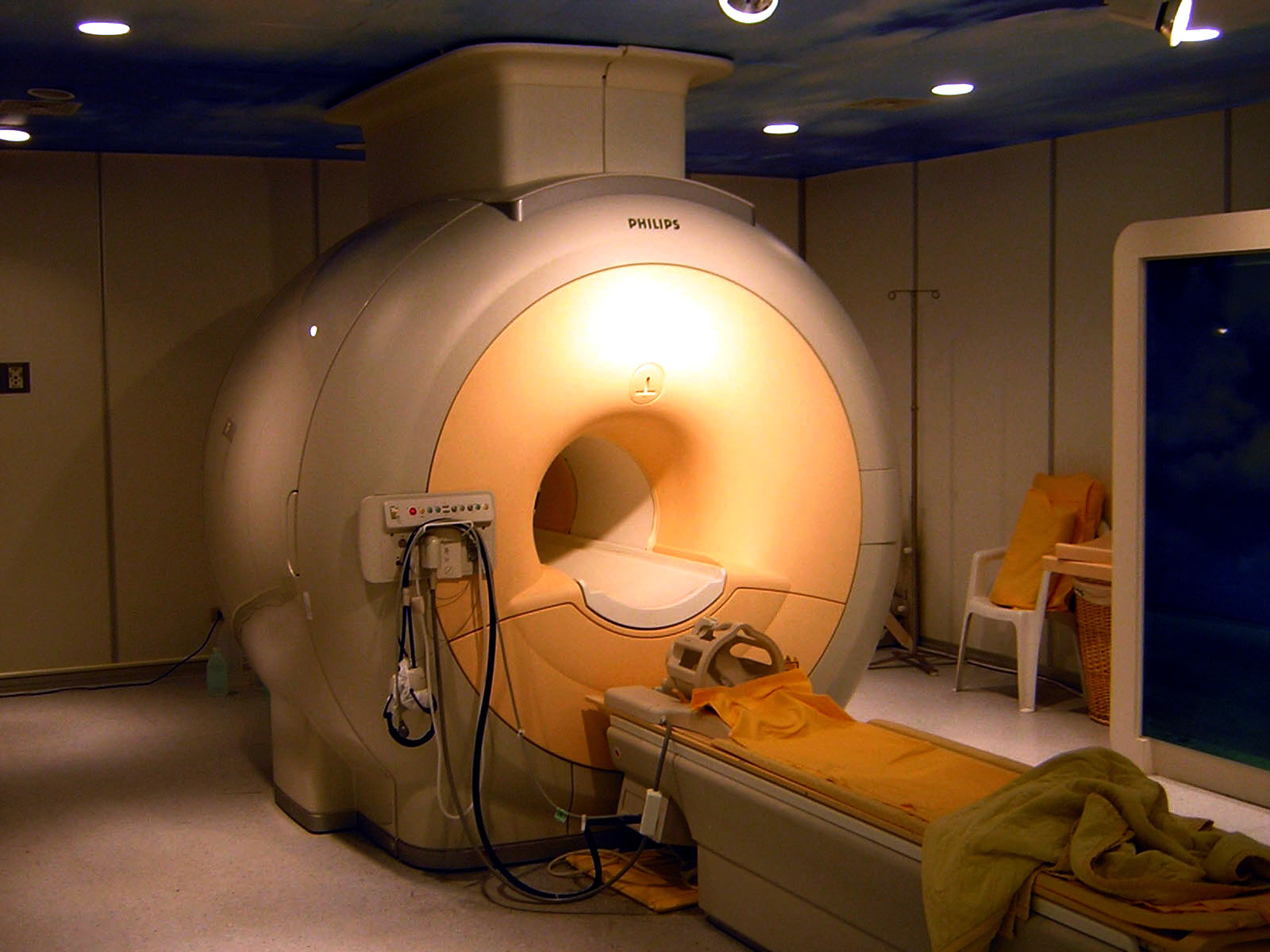 Modern 3T (3 Tesla) MRI scanner, with magnetic field strength 60,000 times that of Earth's magnetic field
⚠️ An Interesting Controversy
Raymond Damadian believed he should have shared the 2003 Nobel Prize because he was the first to prove MRI's medical value. He even placed full-page advertisements in The New York Times and other media to protest. However, the Nobel Committee believed that Lauterbur and Mansfield's contributions were more fundamental—without their spatial encoding technology, MRI imaging would not have been possible at all. This controversy remains a topic in the history of science to this day.
🔬 How Does MRI "See" the Human Body?
Hydrogen Nuclei: "Little Magnets" Inside the Human Body
MRI's imaging principle is completely different from CT—it doesn't rely on X-rays, but rather utilizes the most abundant element in the human body—hydrogen.
Why Choose Hydrogen?
- The human body is about 60% water (H₂O), and fat also contains abundant hydrogen atoms
- Hydrogen nuclei (protons) are magnetic, like tiny magnets
- Hydrogen nuclei have the strongest magnetic resonance signal and are easiest to detect
💡 A Vivid Analogy
Imagine billions of little spinning tops (hydrogen nuclei) inside the human body, normally spinning in all directions. When you place the human body in a strong magnetic field, these little tops align in the same direction like soldiers hearing a command. Then, using a radiofrequency pulse (like a "push"), you knock them over, and as they return to their original state, they emit signals—this is the signal MRI detects.
Four Key Steps of MRI Imaging
1. Apply Strong Magnetic Field (B₀)
- Place the patient in a strong magnetic field (typically 1.5T or 3T)
- Hydrogen nuclei align along the magnetic field direction like compasses
- Form a small net magnetization vector
2. Radiofrequency Pulse Excitation
- Emit radiofrequency pulses at a specific frequency (typically tens of MHz)
- Hydrogen nuclei absorb energy and are "knocked over" (deviate from equilibrium position)
- This frequency is called the "Larmor frequency"
3. Relaxation Process
- After turning off the radiofrequency pulse, hydrogen nuclei gradually return to equilibrium
- Release energy during recovery, producing MRI signal
- Different tissues recover at different rates, which is the source of MRI contrast
4. Spatial Localization
- Use gradient magnetic fields to spatially encode the signal
- Reconstruct images through complex mathematical transformations (Fourier transform)
- Finally obtain axial, coronal, or sagittal images of the human body
T1 and T2 Relaxation: The "Language" of MRI
The most magical aspect of MRI is that by adjusting scanning parameters, it can obtain images with different "contrast." This mainly depends on two relaxation processes:
T1 Relaxation (Longitudinal Relaxation)
- The rate at which hydrogen nuclei return to equilibrium
- T1-weighted images: Fat appears as high signal (bright), water appears as low signal (dark)
- Suitable for observing anatomical structures
T2 Relaxation (Transverse Relaxation)
- The rate at which phase coherence between hydrogen nuclei is lost
- T2-weighted images: Water appears as high signal (bright), fat appears as medium signal
- Suitable for observing lesions (such as edema, tumors)
📊 Clinical Significance of T1 and T2
| Tissue Type | T1-weighted | T2-weighted | Clinical Application |
|---|---|---|---|
| Fat | High signal (bright) | Medium signal | Anatomical structure |
| Water/CSF | Low signal (dark) | High signal (bright) | Edema, effusion |
| Gray Matter | Medium signal | Medium signal | Brain tissue contrast |
| White Matter | High signal | Low signal | Demyelinating lesions |
| Tumor | Low-medium signal | High signal | Tumor detection |
Fundamental Differences Between MRI and CT
| Feature | CT | MRI |
|---|---|---|
| Imaging Principle | X-ray attenuation | Hydrogen nuclear magnetic resonance |
| Radiation | Ionizing radiation | No radiation |
| Soft Tissue Contrast | Poor | Excellent |
| Bone Imaging | Excellent | Poor |
| Scan Speed | Fast (seconds) | Slow (minutes) |
| Contraindications | Caution for pregnant women | Metallic implants in body |
| Cost | Lower | Higher |
⚠️ MRI Contraindications
Due to MRI's use of strong magnetic fields, MRI examination cannot be performed in the following situations:
- Cardiac pacemakers
- Cochlear implants
- Certain metallic implants (such as aneurysm clips)
- Intraocular metallic foreign bodies
- Early pregnancy (caution in first 3 months)
However, many modern implants are "MRI-compatible," and specific consultation with a doctor is needed.
📈 Evolution of MRI Technology
Technology Evolution Timeline
| Era | Milestone Events | Magnetic Field Strength | Scan Time | Main Applications |
|---|---|---|---|---|
| 1970s | Proof of concept stage | - | Hours | Laboratory research |
| 1971: Damadian discovered tumor NMR signal differences | ||||
| 1973: Lauterbur published first MRI image | ||||
| 1977: First whole-body MRI scanner "Indomitable" | ||||
| 1980s | Clinical application begins | 0.15T - 0.5T | 30-60 minutes | Brain, spine |
| 1980: First commercial MRI scanner launched | ||||
| 1990s | High-field popularization | 1.5T | 15-30 minutes | All body organs |
| 1990: Seiji Ogawa discovered BOLD effect (fMRI born) | ||||
| 1.5T became clinical "gold standard" | ||||
| 2000s | Higher field strength & fast imaging | 3T | 10-20 minutes | Functional imaging, spectroscopy |
| 1999: SENSE parallel imaging technology | ||||
| 2002: GRAPPA parallel imaging technology | ||||
| 2010s | Ultra-high field & AI | 7T+ | 5-15 minutes | Research, ultra-early diagnosis |
| Compressed sensing introduced to MRI | ||||
| 7T MRI entered clinical research |
🎯 Interesting Facts About Early MRI
Early MRI scans were very time-consuming, requiring patients to remain still in a narrow scanner for up to 1 hour. Many patients couldn't complete the examination due to claustrophobia. Some hospitals even needed to use sedatives for patients. This also drove the development of "open MRI" and fast imaging technologies.
Key Technology Breakthrough Comparison
| Technology Category | Technology Name | Proposed Time | Core Contribution | Performance Improvement |
|---|---|---|---|---|
| Fast Imaging | Echo Planar Imaging (EPI) | 1970s | Complete image from single excitation | Scan time <100 milliseconds |
| Parallel Imaging | SENSE | 1999 | Utilize multi-channel coil spatial information | Scan time reduced 2-4x |
| Parallel Imaging | GRAPPA | 2002 | k-space self-calibrated parallel acquisition | Scan time reduced 2-4x |
| Sparse Sampling | Compressed Sensing (CS) | 2010s | Utilize image sparsity to reduce sampling | Further reduce scan time |
| Hardware Improvement | Multi-channel coils | 2000s | 8-channel→32-channel→64-channel | SNR greatly improved |
| Hardware Improvement | Enhanced gradient system | 1990s-2000s | Faster switching speed | Spatial resolution improved |
Functional MRI (fMRI): Seeing the Brain "Think"
Revolutionary Breakthrough (1990):
- Discoverer: Seiji Ogawa
- Principle: Blood Oxygen Level Dependent (BOLD) effect - brain activity areas have increased blood flow, changing oxygenated hemoglobin ratio
- Significance: Non-invasive observation of brain functional activity
Main Application Areas:
| Application Area | Specific Applications | Clinical/Research Value |
|---|---|---|
| Clinical Medicine | Preoperative brain function localization (language, motor areas) | Reduce surgical risk, protect important functional areas |
| Cognitive Neuroscience | Memory, attention, emotion and other cognitive process research | Understand brain working mechanisms |
| Mental Disorders | Depression, schizophrenia, autism research | Find biomarkers, guide treatment |
| Brain-Computer Interface | Decode brain activity signals | Assist paralyzed patients in communication |
🧠 Limitations of fMRI
Although fMRI is very powerful, it measures blood flow changes, not neuronal activity itself. Temporal resolution is low (seconds), and spatial resolution is also limited (millimeters). Therefore, it's more suitable for studying "where" activity occurs, rather than "how" it occurs.
Magnetic Field Strength Evolution and Applications
| Magnetic Field Strength | Era | Main Features | Typical Applications | Usage Scenarios |
|---|---|---|---|---|
| 0.15T - 0.5T | 1980s | Low field, slow scanning | Basic brain, spine imaging | Early clinical exploration |
| 1.5T | 1990s-present | Clinical "gold standard" | Routine imaging of all body organs | Most widespread clinical application |
| 3T | 2000s-present | 2x SNR improvement | Functional imaging, spectroscopy, vascular imaging | High-end clinical & research |
| 7T | 2010s-present | Ultra-high resolution (sub-millimeter) | Brain science research, ultra-early lesions | Mainly for research |
| 9.4T - 11.7T | Under development | Extreme exploration | Animal experiments, basic research | Pure research purposes |
⚠️ Challenges of Ultra-High Field MRI
7T and higher ultra-high field MRI, while having extremely high resolution, face many challenges:
- Extremely high cost: Equipment and maintenance costs are several times that of 3T
- Technical complexity: RF field inhomogeneity, increased specific absorption rate (SAR)
- Safety considerations: Stronger magnetic fields require stricter assessment of effects on implants and physiological effects
- Limited clinical application: Currently mainly used for research, routine clinical application still being explored
🎯 Clinical Significance of MRI Technology Evolution
Each advancement in MRI technology has greatly expanded clinical diagnostic and research capabilities:
| Evolution Dimension | Early MRI | Modern MRI | Clinical Significance |
|---|---|---|---|
| Soft Tissue Contrast | Better than CT | Ultimate contrast | From "visible" to "clear" |
| Scan Objects | Brain, spine | All body organs | From "local imaging" to "whole-body imaging" |
| Imaging Capability | Morphological imaging | Morphology + function + metabolism | From "anatomical diagnosis" to "functional diagnosis" |
| Scan Time | 30-60 minutes | 5-15 minutes | From "unbearable" to "routine examination" |
💡 Key Takeaways
Historical Significance: MRI's development went through a long process from physics discovery (1946 NMR) to medical application (1970s-1980s), exemplifying multidisciplinary integration.
Imaging Principle: MRI utilizes the magnetic resonance phenomenon of hydrogen nuclei, generating tissue contrast through differences in T1 and T2 relaxation times, with no ionizing radiation involved.
Technology Evolution: From early low-field, long-duration scanning to modern high-field (1.5T/3T), fast imaging, MRI's clinical practicality has continuously improved.
Unique Advantages: MRI has unparalleled advantages in soft tissue contrast, multi-parametric imaging, and functional imaging, making it the preferred imaging modality for neurology, musculoskeletal, cardiovascular, and other fields.
Future Direction: Ultra-high field MRI (7T+), AI-assisted imaging, real-time MRI, and other technologies will further expand MRI's application boundaries.
💡 Next Steps
Now you understand the basic principles and technological evolution of MRI. In Chapter 3, we will delve into the mathematical principles of MRI image reconstruction, including k-space, Fourier transform, and other core concepts. In Chapter 2, we will learn MRI raw data preprocessing methods, including motion correction, bias field correction, and other practical techniques.