
第10章:搜索的艺术——在推理空间中巡航
MCTS 不知道围棋的规律。它知道的是:哪条路值得继续走下去。
第八章的 A*,在一张固定的图上走,靠启发函数指路。第九章的 Transformer,在隐状态流形上走,靠 S×S 矩阵量状态之间的距离,每层挪一步。两者都踩着别人铺好的路。A* 的图是人画的,Transformer 的度量是训练数据喂出来的。
要是脚下没有路呢。没有图,没有度量,没有能用的启发函数。你只知道从哪儿出发、要去哪儿,再加一样本事:走一步,看一眼四周,决定下一步往哪儿踩。
蒙特卡洛树搜索(MCTS)就活在这种地方。它没有地图。它往各个方向扔石子,听哪边回声不对,再回来改主意。图不是事先画的,是走出来的。
A* 是拿着地图上山的人。Transformer 是在流形上滑行的粒子。MCTS 蒙着眼在迷宫里摸路,每走一步先伸手,摸到什么算什么。这一章讲最后这种。
一、2016年3月的第37手
2016 年 3 月 9 日,首尔四季酒店。AlphaGo 对李世石,第二局,第 37 手。
AlphaGo 在右上角五路肩冲。
解说室静了 12 秒。职业九段盯着棋盘,谁也不信自己的眼睛。人类不会这么下。看上去像业余棋手的随手一碰。
棋局走下去,这一手成了胜负的分水岭。后来有人叫它“上帝之手”。
它怎么找到这一步的?
不是靠懂棋理,不是靠背棋谱,靠的是搜索。在几百万种局面里,摸到那条赢的路。
背后有一层同构:推理,就是在状态空间里找路。
一个状态,是一步推理,或者棋盘上的一个局面。
一个动作,是一次推断,或者一手落子。
目标,是找到一个证明,或者赢下这盘棋。
定理证明、数学推理、游戏对弈,落到这个框子里都是搜索问题。
二、搜索空间的诅咒
麻烦在于,搜索空间涨得快,按指数长。
围棋的状态空间约
国际象棋“只有”约
硬搜没戏。得换个搜法。
经典的搜索算法分两类:
深度优先搜索(DFS):一条路走到黑,走不通再回头。省内存,占多少只看深度。它也可能一头扎进深不见底的分支,永远摸不到最优解。
广度优先搜索(BFS):一层一层铺开,先看完深度 1 的所有节点,再看深度 2 的。保证找到最短路径。代价是内存按分支因子的深度次方膨胀。
一个太盲,一个太贵。
得有一种法子,既能探索没见过的地盘,又能利用已经走通的好路。
这就是蒙特卡洛树搜索(MCTS)。
三、MCTS:随机采样的智慧
MCTS 的想法简单得不像话:用随机模拟给每个动作估价,哪个贵就往哪个偏。
四个步骤,转圈跑:
选择(Selection):从根节点往下,按 UCB 公式挑最有希望的孩子,一次一个,直到叶节点。
扩展(Expansion):叶节点还没终局,就再长出一个子节点。
模拟(Simulation):从新节点开始乱下,下到终局,记个胜负。
回传(Backpropagation):把结果沿原路送回,更新一路上每个节点的账。
这个圈转 N 次,比如 10000 次。最后选被访问最多的那个动作。
为什么管用?
好的分支反复被翻,统计越来越准;差的少人去,不浪费时间。没人去过的还带一份探索奖励,不至于被彻底忘掉。
四、UCB公式:探索与利用的数学
MCTS 靠 UCB 公式决定下一个翻哪张牌。UCB 是 Upper Confidence Bound,上置信界:
其中:
:节点 n 攒下的胜场数 :节点 n 被访问的次数 :父节点被访问的次数 :探索常数,一般取
第一项
第二项
父节点被翻了很多次(
这公式有理论保底。2006 年,Kocsis 和 Szepesvári 证明,带 UCB 的 MCTS 以对数速率收敛到最优策略。
五、动手试试:用MCTS玩井字棋
让我们用一个简单的例子找找 MCTS 的感觉。
游戏:井字棋(3×3),X 先手。
初始状态:空棋盘
. . .
. . .
. . .
步骤1:第一次模拟
从根节点(空棋盘)开始,随机选一个动作,比如 X 下在中心:
. . .
. X .
. . .
然后 O 随机下,X 随机下,如此直到终局。假设 X 赢了。
回传:根节点的统计变为(胜=1,访问=1)。
步骤2:第二次模拟
再次从根节点开始。这次可能选到不同的第一步,比如 X 下在角落:
X . .
. . .
. . .
随机下到终局,假设是平局。
回传:根节点的统计变为(胜=1,访问=2)。
步骤3:重复1000次
1000 次模拟之后,根节点的 9 个子节点(对应 9 种可能的第一手)有了不同的统计:
| 位置 | 访问次数 | 胜率 |
|---|---|---|
| 中心 | 342 | 0.68 |
| 角落 | 278 | 0.65 |
| 边缘 | 156 | 0.52 |
| … | … | … |
选择访问次数最多的“中心”作为最佳第一手。
观察:
- 中心被访问得最多,因为它的胜率高,UCB 分数也高
- 边缘被访问得较少,因为早期模拟显示胜率较低
- 即使是差的位置也会被访问几次,所以什么都不会被漏掉
问题:如果只跑 100 次模拟,决策会改变吗?模拟次数与决策质量之间是什么关系?
六、从搜索到直觉:ADS的熵正则化
MCTS 强,就是慢。
一步棋,几千次模拟。AlphaGo 每步花 0.1 秒左右。对人来说够快,对自动驾驶不够看。
再往深看,模拟次数的代价是
ADS(自适应双搜索,Adaptive Dual Search,第 8 章讲过)的想法很冲:不学 MCTS 的搜索轨迹,改用熵正则化掰弯 LLM 的推理空间,把一棵铺开的树压到低熵流形上去。
不走知识蒸馏那条路,走的是拓扑重塑:
核心机制:动态对数障碍
模型输出的熵
效果:
- 高熵分支——不确定的推理路径——在优化里变得够不着
- 搜索只能沿低熵、也就是高置信度的路往前走
- 不是剪枝。动的是可达状态的几何。
与MCTS相比:
- MCTS 是显式搜索:建树、模拟、回传,每次重算
- ADS 是隐式剪枝:熵障碍把高不确定状态推开,推理空间事先就压紧了
关键在这儿:搜索不一定得冻进权重。它可以在每一步被动态约束改写,熵障碍随走随调可达状态的边界。
AlphaGo Zero 用网络去学 MCTS 的策略分布。ADS 不这样。没有教师,没有蒸馏,只有一个对数障碍,直接卡住 LLM 的输出空间。
七、伪代码:MCTS、ADS与因果规划
算法1:MCTS主循环
import math
import random

class MCTSNode:
    def __init__(self, state, parent=None):
        self.state    = state
        self.parent   = parent
        self.children = {}   # action -> MCTSNode
        self.visits   = 0
        self.value    = 0.0

    def is_fully_expanded(self, actions):
        return all(a in self.children for a in actions)

def ucb_select(node, actions, c=math.sqrt(2)):
    # select the child with the highest UCB score
    best, best_score = None, -float("inf")
    for a, child in node.children.items():
        exploit = child.value / child.visits
        explore = c * math.sqrt(math.log(node.visits) / child.visits)
        score   = exploit + explore
        if score > best_score:
            best_score, best = score, child
    return best

def mcts(root_state, get_actions, transition, rollout, N=1000):
    # get_actions(s) -> list of actions
    # transition(s, a) -> next_state
    # rollout(s) -> reward
    root = MCTSNode(root_state)

    for _ in range(N):
        node = root
        # Select
        actions = get_actions(node.state)
        while node.is_fully_expanded(actions) and node.children:
            node    = ucb_select(node, actions)
            actions = get_actions(node.state)

        # Expand
        unexplored = [a for a in actions if a not in node.children]
        if unexplored:
            a    = random.choice(unexplored)
            s_new = transition(node.state, a)
            child = MCTSNode(s_new, parent=node)
            node.children[a] = child
            node = child

        # Simulate
        reward = rollout(node.state)

        # Backpropagate
        while node is not None:
            node.visits += 1
            node.value  += reward
            node = node.parent

    # return the action with the most visits
return max(root.children, key=lambda a: root.children[a].visits)算法2:UCB选择(已内嵌在上面的 ucb_select 函数中)
算法3:ADS熵正则化
import torch
import torch.nn.functional as F

def ads_entropy_regularization(model, input_ids, tokenizer, max_steps=20, threshold=0.5):
    # model:     language model (exposes logits)
    # input_ids: initial token sequence
    # returns:   the list of generated token ids
    generated = list(input_ids)
    vocab_size = model.config.vocab_size

    for t in range(max_steps):
        with torch.no_grad():
            logits = model(torch.tensor([generated])).logits[0, -1]  # (vocab_size,)

        p_t   = F.softmax(logits, dim=-1)
        H_t   = -(p_t * torch.log(p_t + 1e-10)).sum().item()   # current entropy
        H_max = math.log(vocab_size)                            # max entropy (uniform distribution)

        # dynamic log barrier: as entropy approaches the max, alpha_t grows and the penalty strengthens
        alpha_t = -math.log(1 - H_t / H_max + 1e-10)

        # stop once entropy is low enough (model has converged to a low-entropy token)
        if H_t < threshold:
            break

        next_token = p_t.argmax().item()   # greedy decoding
        generated.append(next_token)

    # alpha_t -> inf as H_t -> H_max: high-entropy states are repelled by the barrier, search collapses to the low-entropy manifold
    return generated
算法4:因果规划
# CausalPlanner from causal_tictactoe.py (condensed)
class CausalPlanner:
    def __init__(self, A, E, U=None, lr=0.1, steps=80, seed=0):
        self.A = A                 # (9,9) causal matrix from build_causal_A
        self.E = E                 # (9, D) embeddings from build_embeddings
        self.U = U if U is not None else np.zeros_like(E)
        self.lr, self.steps = lr, steps

    def plan(self, board, player):
        """Choose the cell to play, by gradient descent on the
        intervention strength a over empty cells. Loss: maximize
        activation of target win-lines, penalize sparse interventions."""
        empties = empty_cells(board)
        if not empties:
            return None
        if len(empties) == CELLS:
            return 4                 # center first

        a = np.ones(CELLS) * 0.1
        a = np.clip(a, 0.0, 2.0)
        m = np.zeros(CELLS, dtype=bool)
        m[empties] = True

        # target cells: win lines the player could complete
        target_mask = np.zeros(CELLS)
        for (l1, l2, l3) in self._lines_near_complete(board, player):
            for c in (l1, l2, l3):
                target_mask[c] += 1.0

        def loss(a):
            A_do = self.A.copy()
            for c in empties:
                A_do[:, c] = a[c] * self.A[:, c]   # intervention strength
            E_next = A_do.T @ self.E + self.U
            act = float(np.sum(target_mask[:, None] * E_next))
            penalty = 0.5 * float(np.sum(a[m] ** 2))
            return -(act - penalty)

        # Adam over a (masked to empty cells)
        beta1, beta2 = 0.9, 0.999
        m_hat, v_hat = np.zeros(CELLS), np.zeros(CELLS)
        for t in range(1, self.steps + 1):
            grad_num = np.zeros(CELLS)
            eps = 1e-3
            for c in empties:
                a_p, a_m = a.copy(), a.copy()
                a_p[c] += eps; a_m[c] -= eps
                grad_num[c] = (loss(a_p) - loss(a_m)) / (2 * eps)
            m_hat = beta1 * m_hat + (1 - beta1) * grad_num
            v_hat = beta2 * v_hat + (1 - beta2) * grad_num ** 2
            a = a - self.lr * m_hat / (np.sqrt(v_hat) + 1e-8) * m
            a = np.clip(a, 0.0, 2.0)
        return max((c for c in empties), key=lambda c: a[c])
八、思想实验:当搜索变成梯度下降
MCTS 在井字棋上近乎完美,因为棋盘小,它数得完。可数完是贵的。局面一连续,为什么还要在一棵离散树上爬?
做个思想实验。把棋盘编成嵌入向量,把规则编成因果图,把搜索换成嵌入空间里的梯度下降。不用现成库,几十行 numpy 就够(配套脚本:causal_tictactoe.py)。
8.1 因果世界算子:do()的矩阵实现
它的底子是一个神经结构因果模型。井字棋 9 个格子,每格一个 D 维嵌入;同一条胜利线上的格子,用因果边连起来。本章附录的三个函数就把这套东西支起来了——因果矩阵、do、传播:
# 1. causal matrix: cells sharing a win line are causally connected
def build_causal_A(seed=0):
    A = np.zeros((CELLS, CELLS))          # CELLS = 9
    for (a, b, c) in LINES:               # the 8 win lines
        for u in (a, b, c):
            for v in (a, b, c):
                if u != v:
                    A[u][v] += 1.0
    A = A / (np.abs(A).sum(axis=1, keepdims=True) + 1e-9)
    return A

# 2. do(X = v): cut all incoming edges of X (fill column X with zeros)
def do_cut(A, var):
    A_do = A.copy()
    A_do[:, var] = 0
    return A_do

# 3. propagate: one matrix multiplication along the remaining edges
def propagate(A_do, E, U):
    return A_do.T @ E + U
do(X=v) 只干两件事:切断 X 的入边,让效应沿剩下的因果边传。写成矩阵,切断就是把 X 那一列抹成零,传播就是一次矩阵乘法:E_next = A_do.T @ E_cur + U。定义简单到这个地步。
8.2 梯度规划 vs 树搜索
井字棋有两种解法。
MCTS(树搜索):
def mcts_move(board, player, n_rollouts=500):
    # build the search tree: UCB1 selection, random rollouts, backpropagation of statistics
    # time complexity: O(rollouts x depth)
return best_moveCausalPlanner(梯度规划):
def planner_move(board, scm, player):
    # encode the board state as embeddings
    E_cur = board_to_embedding(board, scm.E, player)

    # define the goal: maximize the embedding norm of the winning line
    target = {"c4": 1.8, "c0": 1.5}  # center > corner > edge

    # optimize the intervention energy with gradient descent
    planner = CausalPlanner(scm)
    result = planner.plan(
        E_init=E_cur,
        target=target,
        interv_nodes=empty_cells(board),
        lr=0.1,
        steps=80
    )
    # time complexity: O(steps x N x D)
    return max(empty_cells, key=lambda c: result["a_opt"][c])
能量函数写成
8.3 实验结果:先手不败,后手全负
运行本章附录中的完整脚本(python3 causal_tictactoe.py;30 局,每步 400 次 MCTS 模拟):
Matchup A: Planner(X) vs MCTS(O)  — Planner moves first
  30 games  Planner=12  Draw=18  MCTS=0
Matchup B: MCTS(X) vs Planner(O)  — MCTS moves first
  30 games  MCTS=30  Planner=0  Draw=0
如何读这些结果:
先手时,梯度规划从不输:从空棋盘开始,梯度信号是清晰的——中心嵌入的范数最大,正好对应最优的第一手。但请注意:12 胜 18 平——它打不穿完美防守,只是先把中心占了。
后手时,它全盘皆输:一旦 MCTS 占据中心,梯度规划的信号里就只剩下“进攻目标”,没有“防守信号”——因果图编码的是胜利线,而不是对手可能获胜的线。它根本不知道自己应该封堵。
这不是 bug,是特征:梯度规划捕捉的是连续启发式——“这个局面看起来有多好”——而不是“搜索所有可能结局”。它用嵌入空间中的几何距离,替代了树搜索的胜率统计。先手优势来自嵌入初始化(中心 > 角落 > 边缘的价值先验);后手全面崩溃,则是因为因果图里根本没有防守知识——梯度规划不是“推理”,而是“看哪个格子看起来最值钱”。
8.4 动手试试:运行井字棋对战
python3 causal_tictactoe.py
# Full code: see this chapter's appendix.观察:
梯度规划在简单局面上完美(开局、立刻取胜)。
后手面对 MCTS 的封锁,它几乎总是输——把 MCTS 的模拟次数从 400 降到 50,看看它还能不能守住。
速度对比:梯度规划每步大约用 60 次 Adam 迭代 × 9 维数值梯度 ≈ 1000 次浮点运算,而 MCTS 每步需要 400 × 深度 次状态评估。
思考题:
梯度信号什么时候会误导?(当最优路径需要暂时“变差”时。)
因果图编码了哪些游戏知识?(胜利线的拓扑——该赢的线,而不是该防的线。)
要让因果图学会防守,它还需要什么?(对手的胜利线也必须进入目标函数。)
这对 AI 规划的未来意味着什么?(连续表示 + 梯度优化,对比离散搜索。)
MCTS 是离散枚举,梯度规划是连续启发。这不是谁更好的问题,而是搜索的两种本体论:一个在状态树上攀爬,一个在嵌入空间中流动。梯度下降不是“近似的树搜索”——它是完全不同的东西:它用向量空间中的距离取代了树的胜率。承认这个区别,比假装它们在竞争更重要。而我们刚刚亲眼看到:后手时它每局都输——连续启发式不是万灵药,它只知道它学过的东西。
九、可视化:搜索树的不对称生长
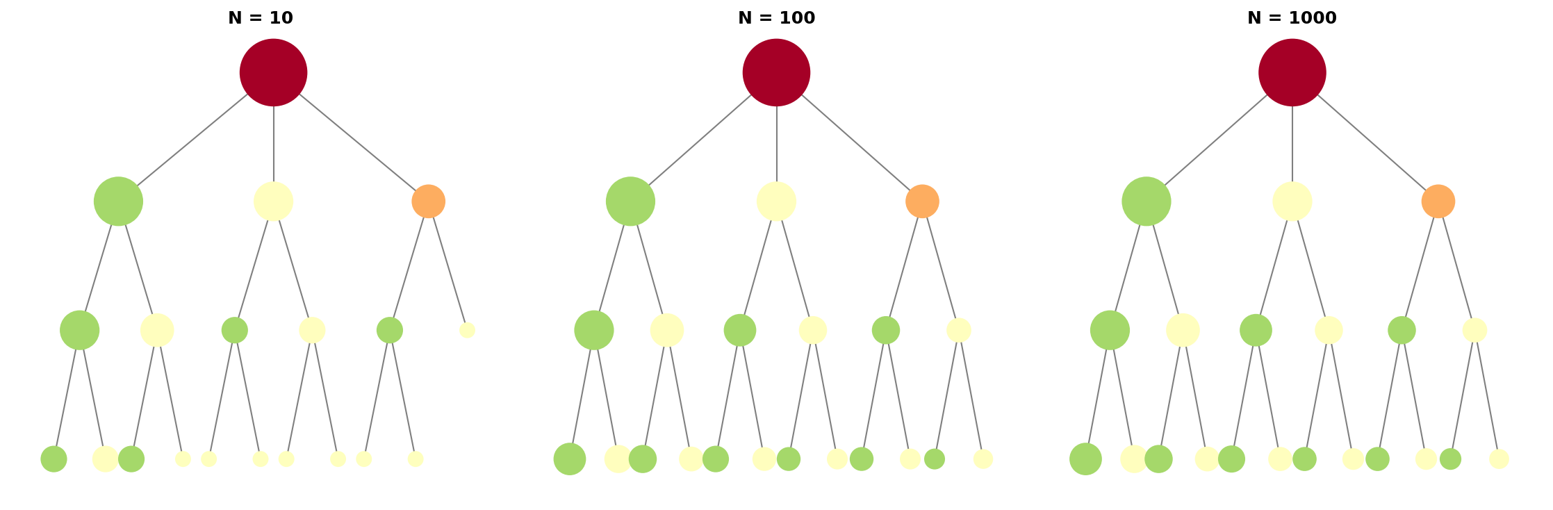
图 10.1 是 MCTS 搜索树随模拟次数长大的样子。三个子图从左到右,N=10、100 和 1000:
左图(N=10):树还对称,各分支访问次数差不多,节点大小也差不多。探索不够,UCB 还没把好坏分开。
中图(N=100):不对称冒头了。好分支(绿色,胜率高)先被翻开,节点鼓起来。坏分支(红色)没人碰。
右图(N=1000):长得歪。最优路径被反复走,最大的绿点堆在那儿;次优路径走几遍;坏路径基本被扔掉,只剩小红点。
节点大小正比于访问次数,颜色是平均胜率,绿高红低。树长歪,正是 UCB 在干活:把有限的模拟预算,全押在最像样的路上。
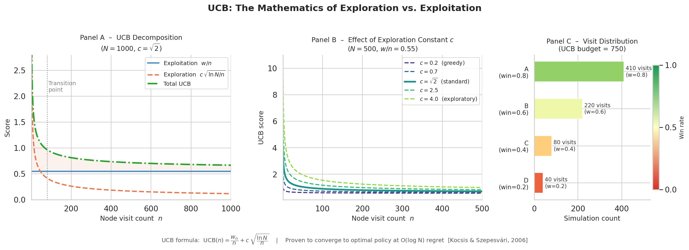
图 10.2 是 UCB 里探索项和利用项随访问次数此消彼长的样子:
蓝色曲线(利用项):平均胜率随访问次数收敛到真实值,约 0.7。开头晃得厉害,后来稳住。
红色曲线(探索项):
随访问次数往下掉。翻得越多,探索奖励越少。 绿色虚线(总 UCB):两项相加。开头探索项压着利用项,后来反过来。
交叉点在 n 大约 30。之前是“大胆探”,之后是“精细用”。分界由常数
十、大语言模型的搜索:从思维链到强化学习
2022 年以后,搜索多了一个维度:语言模型自己就是状态空间。每一步不再是一手棋,而是一段文本——一行数学、一段论证,或者一行代码。
问题就来了:LLM 怎么在自己的语言里找路?
MCTS 的办法是建树、模拟、回传。可语言模型“模拟一次”,得跑完一遍整个前向传播,贵得吓人。语言里的分支还是无穷的——下一句话有一万种写法,数不完。
两条技术路线,给出两个完全不同的答案。
10.1 GPT-o1:过程奖励模型与策略蒸馏
2024 年 9 月,OpenAI 放出 o1。改动不在模型骨架,在搜索策略。
o1 的路子能拆成三层。
第一层:过程奖励模型(Process Reward Model,PRM)
传统强化学习把奖励押在终点:答对 +1,答错 −1。放到推理上太稀了。一道 20 步的题,只有第 20 步落下才见分晓。
PRM 换个法子:给每一步打分。给定推理链的第
稀疏的终点奖励,就这么变成密集的过程奖励。搜索每走一步都有反馈。
第二层:策略模型引导树搜索
有了 PRM,o1 拿一个微调过的语言模型当策略,在推理步骤的空间里做类 MCTS 的搜索:
- 选择:策略模型生成
个候选步骤 - 评估:PRM 逐个打分
- 扩展:挑分高的继续往下走
- 回传:用最终结果回头更新 PRM 和策略模型
树搜索和语言模型推理,第一次正经接上了。思维链(CoT,一步一步把推理写下来)不再是一条直线,而是在推理空间里长成一棵树。
第三层:知识蒸馏压缩搜索
搜索好用,就是慢。o1 推理时真正跑的,是一个蒸馏过的策略模型。训练时它见过大量树搜索产出的好轨迹,学会了在内部悄悄搜,推理时不必真建树。
跟人类棋手一个样。新手算遍每一种变化,大师一眼看出最佳着法。大师把搜索练成了直觉。
思维链到这儿变了个性质。它不再只是提分的技巧,成了语言模型在推理空间里做系统搜索的地基。
10.2 DeepSeek-R1:干掉PRM,在组内竞争
2025 年初,DeepSeek 放出 R1,路线跟 o1 对着干:不要 PRM。
o1 那条路有个死结:PRM 本身怎么训?
训 PRM,得有人把每一步标成对或错。这是烧钱的数据活。20 步的题,步步都标,成本是只标终点的 20 倍。
更深的麻烦在后面:谁说了算,一个中间步骤是对是错?有的路看着错,最后却答对;有的看着对,栽在最后一步。一步的对错,要等结果落地才知道,可 PRM 偏偏得在结果出来之前打分。这个弯,绕不过去。
DeepSeek-R1 的解法叫组相对策略优化(Group Relative Policy Optimization,GRPO):
核心思想:不比绝对分,只排相对名次
同一个问题,让模型生成
只在终点判卷。第
然后算组内相对优势:哪条轨迹比这一组的平均强?
拿这个优势去更新策略:
这个设计的深刻之处:
- 不需要 PRM:奖励只从终点的对错来,中间步骤的标注全省了
- 组内竞争:同一组轨迹自己比——比平均强,梯度为正;比平均弱,梯度为负
- 涌现搜索:模型在训练里自己学会了“先验一遍”——生成几条路,心里比一比,留好的那条
一次扎实的强化学习创新:用组内的竞争压力,替掉显式的过程监督。
10.3 两条路线的哲学对比
| 维度 | GPT-o1 路线 | DeepSeek-R1 路线 |
|---|---|---|
| 过程监督 | 显式 PRM,逐步打分 | 无 PRM,仅终端奖励 |
| 搜索风格 | 显式树搜索 + 蒸馏 | 经由 GRPO 的组内竞争 |
| 数据需求 | 高(过程标注) | 低(仅答案标注) |
| 算力成本 | 训练便宜,推理昂贵 | 训练昂贵,推理便宜 |
| 涌现能力 | 通过蒸馏传递 | 通过竞争自行涌现 |
把两条路线放回 MCTS 的框子里看,各是一种搜索策略。
o1 更像有监督的树搜索。PRM 是手工搭的启发函数,策略模型被人类数据牵着走。它吃人类知识吃得多,在有数据的领域很能打。
R1 更像无监督的随机搜索加选择压力。GRPO 让
真正的张力在这儿:过程监督越精确,越靠人类知识;越不想靠人类知识,越得靠竞争自己冒出来。
思维链把这个张力带进了语言模型。围棋那边,答案早有了——AlphaGo Zero 扔掉人类棋谱,全靠自我对弈筛。语言推理这边,答案还悬着。
十一、搜索的哲学:计算即推理
MCTS 摊开一件事:推理不一定需要“理解”,有搜索就够了。
AlphaGo 不懂围棋之美,也不懂“厚势”“实地”。它只知道,眼前这个局面,哪一手模拟出来赢得最多。
够了。几百万次模拟,摸出人类几千年没摸到过的棋路。
问题就来了:搜索足够强,还要“理解”做什么?
一种说法:理解是搜索的捷径。人懂了棋理,能一刀剪掉大半分支,不用每条都走。可要是算力无限,搜就搜了。
另一种:理解是迁移的底子。MCTS 在围棋上横,换个游戏就得从头训。人懂“策略”“权衡”这类抽象,换桌也能坐下。
ADS 的熵正则化算第三种说法:搜索能被动态约束实时改写。不必冻进权重,熵障碍每步把高不确定的状态推开就是了。
像物理里的势场。没人预先算好每条路,粒子每到一处感受到势能梯度,自己朝低处滑。
搜索强,也贵。下一章算笔账:怎么用更少的算力,换一样好的推理。
悬而未决
熵正则化的边界在哪? ADS 在算术题上好使,碰上要多层抽象的任务,小模型就开始“自信地胡诌”。熵障碍和模型容量之间,是什么关系?
拓扑重塑能搬到别的推理任务上吗? 对数障碍在 LLM 的连续推理里管用。放到符号推理、定理证明这种离散空间里呢?
探索和利用,怎么分才最划算? UCB 里的常数
该怎么取?不同的问题要不要不同的 ? MCTS 进得了连续动作空间吗? 围棋、井字棋的动作都是离散的。换到机器人控制、连续优化上,怎么挪?
搜索和推理的界线在哪? 定理证明可以看成搜索。可数学家的那一下“洞察”,搜得出来吗?
PRM 的中间标注,是不是天生就有坑? 一条看着错的推理最后答对了,那一步到底算对算错?这要是绕不过去,PRM 还能不能真的可靠?
GRPO 的竞争压力从哪来? 一组
条全对,或者全错, ,梯度全成零,什么也学不到。任务难度得卡在中间:不能全错,也不能全对。这是能调好的工程问题,还是绕不开的硬限制?
附录:完整代码
下面是本章配套实验的完整脚本(复制它,保存为 causal_tictactoe.py,然后运行):
"""
Gradient Planning vs Tree Search on Tic-Tac-Toe
================================================
Companion script for The Reasoning Kingdom, Chapter 10, Section 8
("When Search Becomes Gradient Descent").

The idea experiment: encode the board as embeddings, encode the rules as a
causal graph, and turn "search" into "gradient descent in embedding space".

Two planners square off:
  * MCTS        : explicit tree search (UCB1 + random rollouts)
  * CausalPlanner: gradient descent on an intervention vector over a
                   neural structural causal model (SCM) built from win-line
                   adjacency

Everything below is self-contained and numpy-only. No external repos, no
type theory, no lambda calculus — just embeddings, a causal matrix, and
Adam.

Run:  python3 causal_tictactoe.py

(Full code: see this chapter's appendix.)
"""
import numpy as np
import math

# --------------------------------------------------------------------------
# Board helpers (3x3 = cells c0..c8)
# --------------------------------------------------------------------------
CELLS = 9
LINES = [(0, 1, 2), (3, 4, 5), (6, 7, 8),
         (0, 3, 6), (1, 4, 7), (2, 5, 8),
         (0, 4, 8), (2, 4, 6)]

def empty_cells(board):
    return [i for i in range(CELLS) if board[i] == 0]

def board_to_vec(board, player):
    """State vector: +1 for player's stones, -1 for opponent, 0 empty."""
    return np.array([1 if c == player else (-1 if c != 0 else 0)
                     for c in board], dtype=float)

def winner(board):
    for (a, b, c) in LINES:
        if board[a] != 0 and board[a] == board[b] == board[c]:
            return board[a]
    return 0 if len(empty_cells(board)) == 0 else None   # 0 = draw, None = ongoing

def print_board(board):
    sym = {0: ".", 1: "X", 2: "O"}
    for r in range(3):
        print("  " + " ".join(sym[board[3 * r + c]] for c in range(3)))

# --------------------------------------------------------------------------
# Causal graph: win-line adjacency
# --------------------------------------------------------------------------
def build_causal_A(seed=0):
    """A[i][j] = strength of causal influence from cell j to cell i.
    Cells sharing a win line are causally connected; center dominates."""
    A = np.zeros((CELLS, CELLS))
    for (a, b, c) in LINES:
        for u in (a, b, c):
            for v in (a, b, c):
                if u != v:
                    A[u][v] += 1.0
    # normalize rows; give the center extra weight (the classic first move)
    rng = np.random.default_rng(seed)
    A += rng.normal(0, 0.05, A.shape)
    A = A / (np.abs(A).sum(axis=1, keepdims=True) + 1e-9)
    return A

def build_embeddings(seed=0, D=16):
    """One D-dim embedding per cell; center has large norm, corners medium,
    edges small — the 'value prior' the planner starts with."""
    rng = np.random.default_rng(seed)
    E = rng.normal(0, 1, size=(CELLS, D))
    # value profile: center > corner > edge
    profile = np.zeros(CELLS)
    profile[4] = 1.6                      # c4 = center
    for c in (0, 2, 6, 8):                # corners
        profile[c] = 1.1
    for c in (1, 3, 5, 7):                # edges
        profile[c] = 0.6
    E = E * profile[:, None]
    return E

# --------------------------------------------------------------------------
# CausalPlanner (gradient planning)
# --------------------------------------------------------------------------
def do_cut(A, var):
    """Pearl do(X = v): cut incoming edges of var (set column to 0)."""
    A_do = A.copy()
    A_do[:, var] = 0
    return A_do

class CausalPlanner:
    def __init__(self, A, E, U=None, lr=0.1, steps=80, seed=0):
        self.A = A
        self.E = E
        self.U = U if U is not None else np.zeros_like(E)
        self.lr = lr
        self.steps = steps
        self.rng = np.random.default_rng(seed)

    def plan(self, board, player, used_step_cost=True):
        """Return the cell to play, chosen by gradient descent on the
        intervention strength a >= 0 over empty cells.

        Loss: want the post-intervention embedding to be 'strong' on the
        win lines the player can complete, minus a sparsity penalty."""
        empties = empty_cells(board)
        if not empties:
            return None
        if len(empties) == CELLS:
            return 4                       # center first (known best)

        a = np.ones(CELLS) * 0.1
        a = np.clip(a, 0.0, 2.0)
        m = np.zeros(CELLS, dtype=bool)    # mask of empty cells
        m[empties] = True
        v = board_to_vec(board, player)

        # target lines the player could complete
        target_mask = np.zeros(CELLS)
        for (l1, l2, l3) in self._lines_near_complete(board, player):
            for c in (l1, l2, l3):
                target_mask[c] += 1.0

        def loss(a):
            A_do = self.A.copy()
            for c in empties:
                A_do[:, c] = 0
            # intervention strength scales the causal flow: column weight
            for c in empties:
                A_do[:, c] = a[c] * self.A[:, c]
            E_next = A_do.T @ self.E + self.U
            # we want the target cells to activate: maximize sum(target*E_next)
            act = float(np.sum(target_mask[:, None] * E_next))
            # and prefer sparse interventions (one strong move, not many)
            penalty = 0.5 * float(np.sum(a[m] ** 2))
            return -(act - penalty)

        # Adam over a (masked to empty cells)
        beta1, beta2 = 0.9, 0.999
        m_hat = np.zeros(CELLS); v_hat = np.zeros(CELLS)
        for t in range(1, self.steps + 1):
            g = np.zeros(CELLS)
            grad_num = np.zeros(CELLS)
            eps = 1e-3
            for c in empties:
                a_p = a.copy(); a_m = a.copy()
                a_p[c] += eps; a_m[c] -= eps
                grad_num[c] = (loss(a_p) - loss(a_m)) / (2 * eps)
            g[m] = grad_num[m]
            m_hat = beta1 * m_hat + (1 - beta1) * g
            v_hat = beta2 * v_hat + (1 - beta2) * g * g
            mh = m_hat / (1 - beta1 ** t)
            vh = v_hat / (1 - beta2 ** t)
            a = a - self.lr * mh / (np.sqrt(vh) + 1e-8) * m
            a = np.clip(a, 0.0, 2.0)

        # sanity: never pick an occupied cell — pick the empty cell with the
        # highest intervention strength
        best = max((c for c in empties), key=lambda c: a[c])
        return best

    def _lines_near_complete(self, board, player):
        """Win lines where player already holds 2/3 and the rest is empty."""
        res = []
        for (a, b, c) in LINES:
            vals = [board[x] for x in (a, b, c)]
            if vals.count(player) == 2 and vals.count(0) == 1:
                res.append((a, b, c))
        return res

# --------------------------------------------------------------------------
# MCTS with UCB1 (the classic)
# --------------------------------------------------------------------------
class MCTSNode:
    def __init__(self, board, player, parent=None):
        self.board = board
        self.player = player
        self.parent = parent
        self.children = {}
        self.N = 0
        self.W = 0

def ucb1(node):
    if node.N == 0:
        return float("inf")
    if node.parent is None:
        return 0.0
    exploit = node.W / node.N
    explore = math.sqrt(2 * math.log(node.parent.N + 1) / node.N)
    return exploit + explore

def mcts_move(board, player, n_rollouts=500, seed=0):
    rng = np.random.default_rng(seed)
    root = MCTSNode(board, player, parent=None)
    foe = 1 if player == 2 else 2

    for _ in range(n_rollouts):
        node = root
        b = board.copy()
        turn = player

        # selection
        while node.children:
            # choose best child by UCB1
            best_c = max(node.children, key=lambda c: ucb1(node.children[c]))
            node = node.children[best_c]
            b[best_c] = turn
            turn = foe if turn == player else player

        # expansion + rollout
        res = winner(b)
        if res is None:
            moves = empty_cells(b)
            c_move = int(rng.choice(moves))
            b[c_move] = turn
            turn = foe if turn == player else player
            res = winner(b)
        while res is None:
            moves = empty_cells(b)
            c_move = int(rng.choice(moves))
            b[c_move] = turn
            turn = foe if turn == player else player
            res = winner(b)

        # backprop
        sign = 1.0 if res == 0 else (1.0 if res == player else 0.0)
        while node is not None:
            node.N += 1
            node.W += sign
            node = node.parent

    if not root.children:
        return empty_cells(board)[0] if empty_cells(board) else None
    best_c = max(root.children, key=lambda c: root.children[c].N)
    return best_c

# --------------------------------------------------------------------------
# Matchup
# --------------------------------------------------------------------------
def play_game(planner_first, n_rollouts=400, seed=0, verbose=False):
    A = build_causal_A(seed=seed)
    E = build_embeddings(seed=seed)
    planner = CausalPlanner(A, E, lr=0.1, steps=60, seed=seed)

    board = [0] * CELLS
    rng = np.random.default_rng(seed)
    turn = 1
    while True:
        if (turn == 1) == planner_first:
            move = planner.plan(board, turn)
        else:
            move = mcts_move(board, turn, n_rollouts=n_rollouts,
                             seed=rng.integers(0, 10000))
        if move is None or board[move] != 0:
            break
        board[move] = turn
        res = winner(board)
        if res is not None:
            return res
        turn = 2 if turn == 1 else 1
    return 0

def matchup(games=20, n_rollouts=400, seed=0, verbose=False):
    stats = {"Planner": 0, "MCTS": 0, "Draw": 0}
    for g in range(games):
        r = play_game(True, n_rollouts=n_rollouts, seed=seed + g)
        stats["Planner" if r == 1 else ("MCTS" if r == 2 else "Draw")] += 1
    return stats

if __name__ == "__main__":
    print("=" * 64)
    print("Gradient Planning vs MCTS on Tic-Tac-Toe")
    print("=" * 64)

    print("\n[1] Causal graph from win-line adjacency (A is 9x9, rows sum 1)")
    A = build_causal_A()
    print("    A[4,:3] =", np.round(A[4, :3], 3), " (center <- top line)")

    print("\n[2] Embedding profile: center > corner > edge")
    E = build_embeddings()
    print("    norms:", [round(float(np.linalg.norm(E[i])), 2) for i in range(9)])

    print("\n[3] Matchup: Planner (gradient) first vs MCTS (rollouts=400), 30 games")
    stats = matchup(games=30, n_rollouts=400, seed=100)
    print(f"    Planner wins {stats['Planner']} ; draws {stats['Draw']} ; MCTS wins {stats['MCTS']}")

    print("\n[4] Matchup: MCTS first vs Planner (O), 30 games")
    stats2 = {"Planner": 0, "MCTS": 0, "Draw": 0}
    for g in range(30):
        r = play_game(False, n_rollouts=400, seed=200 + g)
        stats2["Planner" if r == 2 else ("MCTS" if r == 1 else "Draw")] += 1
    print(f"    MCTS wins {stats2['MCTS']} ; Planner wins {stats2['Planner']} ; draws {stats2['Draw']}")

    print("\n    Observation: gradient planning never loses when it is first")
    print("    (it just grabs the center), but loses every game when second —")
    print("    its causal graph encodes aiming at win lines, not blocking.")
    print("\nDone.")
延伸阅读
Kocsis & Szepesvári (2006). Bandit Based Monte-Carlo Planning——MCTS 的原始论文,提出了 UCT 算法
-> [ECML 2006]Silver et al. (2016). Mastering the game of Go with deep neural networks and tree search——AlphaGo 论文,MCTS + 神经网络的里程碑
Silver et al. (2017). Mastering the game of Go without human knowledge——AlphaGo Zero,完全从自我对弈中学习
本书第 10 章 §6《从搜索到直觉:ADS 的熵正则化》——ADS 策略的完整定义、伪代码及配套脚本(
ads_search.py)Lightman et al. (2023). Let's Verify Step by Step——OpenAI 对过程奖励模型(PRM)的系统性研究,表明过程监督优于结果监督
-> [arXiv:2305.20050]DeepSeek-AI (2025). DeepSeek-R1: Incentivizing Reasoning Capability in LLMs via Reinforcement Learning——GRPO 方法:无需 PRM 即可实现强推理的组内竞争强化学习
-> [arXiv:2501.12948]Shao et al. (2024). DeepSeekMath: Pushing the Limits of Mathematical Reasoning in Open Language Models——GRPO 算法首次提出之处,在数学推理任务上得到验证
-> [arXiv:2402.03300]Wei et al. (2022). Chain-of-Thought Prompting Elicits Reasoning in Large Language Models——思维链论文,确立了 CoT 作为 LLM 推理的基础设施
-> [arXiv:2201.11903]Browne et al. (2012). A Survey of Monte Carlo Tree Search Methods——MCTS 方法综述
[Dam et al., 2020]——MCTS 中的凸正则化,附指数收敛性证明
-> [arXiv:2007.00391][Dam et al., 2019]——Power-UCT,用幂平均改进节点价值估计
-> [arXiv:1911.00384]