
第12章:隐式推理——神经网络的内部独白
在模型输出第一个 token 之前,它做了什么?
前四章构成了一条搜索的光谱。第 8 章:离散图上的显式搜索(A*、ADS)。第 9 章:隐状态流形上的软搜索,用
但它们共享一个前提:搜索是显式的。你建一棵树。你算一个矩阵。你跑 N 次模拟。模型在“外面”找。
问题换到了“里面”。模型输出第一个 token 之前,显式地“搜索”之前,隐藏层里发生了什么?一次前向传播本身——那
答案的核心是永霖公式:
一、黑盒里的思考
2022 年,Wei 等人试了一件笨办法:让大语言模型(LLM——在海量文本上训练、用来预测下一个词的模型)在给答案之前先把推理说出来。准确率大幅跃升。
这就是思维链(chain of thought,CoT):一步一步推,把步骤写下来。
思维链(CoT):为什么“把步骤说出来”能让模型变聪明?(前人工作:Wei et al., 2022)
思维链(Chain-of-Thought,CoT)提示是 2022 年 Google Brain 的 Wei 等人发现的技巧:在问题后面加一句“让我们一步一步思考”(let us think step by step),或者在少样本示例里摆出推理步骤,模型在复杂任务上的准确率就会往上跳。
为什么有效? 主流的解释是:
- 更大的计算预算:每生成一个 token 都要多走一步计算。让模型把中间步骤写出来,相当于允许它打草稿,而不是逼它心算。
- 每个中间输出都变成新的输入:模型写出的每一步都会追加到上下文里,成为下一步的输入。这就把一个难题拆成了更简单的子问题。
一个重要的限制:CoT 对很小的模型几乎无效;它只在约 1000 亿参数以上才涌现。这说明它依赖某种只有大模型才具备的底层能力。
于是一个问题挂在这儿:模型是在“推理”,还是在“匹配格式”?
例如这个问题:“罗杰有 5 个网球。他又买了 2 罐网球,每罐有 3 个球。他现在有多少个球?”
直接回答:
Model output: 11 balls
Accuracy: 17%
CoT 提示:“让我们一步一步思考”
Model output:
Roger had 5 balls.
He bought 2 cans with 3 balls each, so that's 2×3 = 6 balls.
That's 5+6 = 11 balls in total.
Answer: 11 balls
Accuracy: 78%
17% 到 78%。参数没变,训练数据没变,变的只是模型被要求把中间步骤写出来。
那么,在模型“说出”推理之前,它自己内部发生了什么?
暂停一下
17% 到 78%。只是把步骤说出来的这个动作,计算就变了。
同一个模型,同一套权重,同样多的参数。只多了一条要求:把中间步骤写出来。
这说明什么?
一种解释:能力本来就在,CoT 只是把它放出来,给了模型多走几步计算的机会。
另一种解释:模型根本没推理。它在匹配“推理步骤的格式”。写出“罗杰有 5 个球”之后,这句话成了下一步的输入,题目被改成了统计匹配更顺手的形状。
多数时候,两种解释给出同样的预测。可它们对“模型是什么”的回答,差得很远。
哪一种是真?有没有一个实验能把两者分开?
先搁着。
二、隐层:推理的暗室
前向传播是一层接一层的变换:
第
这些层在干什么?
浅层抓边缘、纹理,深层抓物体、概念——这是感知任务里的说法。放到推理上,事情细一点。
2022 年,Olsson 等人盯上了 GPT 的归纳头(induction heads):一种专门“看见模式,接下一个”的注意力头。
输入序列是“A B C A B ?”。
归纳头看见“A B”又出现了一遍,把下一个 token 押在“C”上。
隐藏层里有一份像工作记忆的东西:模型留着刚才的模式,拿它推下一步。
这份记忆有多深?能撑多长的推理?
三、隐层里到底发生了什么
把问题说得再准一点。
CoT 有用,不是因为它给模型塞进了新的逻辑规则。它把压在一次前向传播里的东西摊开,摊成一串能写下来的中间状态。写出来的是表面;先发生的,还是隐藏层里的状态演化。
答案出口之前,隐藏层干了多少活?这是本章要追的。
最自然的想法:一次前向传播就是一场逐层展开的内部独白。输入不会一步变成答案。它先变成中间表示,再被重组、压缩、放大,最后才投影到输出。写成公式:
每个
感知任务里,浅层看边缘,深层看物体。推理任务里更像:浅层把问题改写成模型能用的坐标,深层在坐标里整合关系。
Olsson 等人在 2022 年对 GPT 的研究,重要就重要在这儿。有些注意力头干的是工作记忆的活:看见一个模式,就持续跟着它。输入“A B C A B ?”,归纳头把前面的“A B”和后面的“A B”对上,下一个 token 押“C”。
重点不是“会补全序列”,那太浅。隐藏层不是静态的特征仓库。它维持一个能操作的内部状态:留住局部关系,对齐远处的片段,把见过的结构带进当下接着算。这已经很像我们说的“中间推理”。
所以问题不是模型有没有想法。问题是这个状态能演化多远。
能撑多步推理吗?一步都不写下来,内部能把逻辑稳稳传下去吗?
永霖公式给的答案不客气:走一阵可以,走不了无限远;对象层能推进,元层认不了自己。临时窗口总会被先验锚点收回去。
说 CoT“教会模型把想法说出来”,不够。CoT 只是让这场内部独白多有用一会儿。
如果里面真有一场独白,链子变长的时候,它从哪里开始失真?
四、CoT:让隐式推理显式化
CoT 干了什么?一种说法:它把隐式推理拽到明面上。
平时,推理发生在隐藏层里,一次前向传播从输入走到输出。这个过程是压缩的:所有步骤挤进有限的层数。
CoT 生成中间 token,换来的其实是计算时间:
- 每生成一个 token,就要多走一次完整的前向传播
- 一条 10 个 token 的推理链,就要走 10 次前向传播
- 这给了模型 10 倍的计算深度
人也这样。题难的时候不立刻答,把步骤写在纸上,一步一步往前挪。
可这里有个分不清的地方:它是在推理,还是在表演推理?
五、永霖公式:先验从哪里来?
永霖公式给 CoT 划了一条底:链子再长,最后都会收回到先验锚点。
公式是这样:
记号先说清楚:这里的
读它之前,先认三个东西:
先验锚点
先验锚点不神秘。它是训练数据的统计偏置。
假设训练集里 50% 是正例(链条完整,答“是”),50% 是负例(链条断裂,答“否”)。
这样的训练集,会让模型学出一个默认倾向:不知道怎么答,就五五开猜。
这个默认倾向就是先验锚点
写成式子:
训练集标签的边缘分布。
训练集 60% 是正例,
这个锚点是模型从数据里吸收来的偏置。不是错误。它是模型对“世界平均长什么样”的最好猜测。
推断分布
:一步没推,分布就是先验 :看见第一条证据,分布更新一次 :处理了 10 个推理步骤 :无限推理后的极限
永霖公式说:推理无穷多步,分布最后也回到
链条完整(A>B>C>…>Z 全成立),“A>Z”的答案就是 100% 的“是”。
模型的极限是
六、隐式推理的哲学意义
永霖公式说的不是哪家的模型没做好。推理本身就不完备。
系统够强,就会撞上元层断裂:
- 它能在对象层生成推理链
- 但无法在元层验证推理链的对错
- 最后只能退回先验锚点
这不是规模的事。GPT-4o 有 2000 亿参数,照样收敛。只是收敛点可能离真实分布近一点(
CoT 能做的是把
这样看,隐式推理(隐藏层内部)和显式推理(CoT 生成 token)是同一件事:都在有限的计算深度里朝正确答案挤。
区别只有一条:
- 隐式推理:压缩在一次前向传播中——快但浅
- 显式推理:展开为多次前向传播——慢但深
两条路都受永霖公式管。都会收敛。
永霖公式画的是推理的内边界。下一章是最后一章,把这些边界拼在一起:推理王国的地图。
七、永霖极限的严格推导:从不动点到压缩映射
1. 从最朴素的不动点概念说起
不动点:最简单的定义。对于函数
定义看似平凡,但它藏着一层很深的哲学:自指。系统的输出等于它的输入;原因等于结果。
2. 迭代一个序列:离散动力系统
考虑一个由递推定义的序列
这是一个离散动力系统。我们想知道:当
2.1 一个具体的例子
最简单的线性情形:
- 不动点方程:
(若 ) - 迭代:
- 解:
- 收敛:当
时,
那个
3. 建立信念空间
在推理系统中,
令
从 {0,1} 到 [0,1]:信念为什么应该是定量的?
在经典逻辑里,一个命题要么真要么假。“明天会下雨”是 1 或 0。状态空间是一组离散的顶点。
但你并不知道哪个是真相。你能知道的只是自己的确信程度。
贝叶斯式的转向:把“世界的状态”换成“你对世界的认知状态”。
- 经典逻辑:
;每个命题为真或为假 - 贝叶斯信念:
;每个命题带一个置信度
那个 0.7 不是“世界有 70% 的概率下雨”,而是你,作为认知主体,对这个命题有 0.7 的置信度。世界本身仍然是 0 或 1——模糊的是你的知识,不是世界。
再加上归一化约束
为什么单纯形是 n-1 维而不是 n 维?
有
但有一个约束:
这个约束移除了一个自由度。你只需要自由选择前
类比:直线上的点是 1 维的,但如果我们约束
具体地:
(二选一):单纯形是 里的一条线段——1 维 (三选一):单纯形是平面上的一个等边三角形——2 维 (四选一):单纯形是空间里的一个正四面体——3 维
每个顶点对应“对某个答案完全确定”(经典逻辑的状态)。内部的点是贝叶斯的领地——一片连续的不确定性光谱。
单纯形的几何本质:凸集的定义里藏着什么?
单纯形不只是一个几何形状;它是凸性的最小单元。
凸集定义:集合
看那个条件:
所以凸集的定义可以重读为:
单纯形是“刚好够用的凸性容器”:
线性规划的单纯形法共享同一套直觉。线性规划在凸多面体(可行域)上最小化一个线性目标。关键事实是:在凸多面体上,线性函数必在某个顶点取到最优值。
单纯形法的策略:从一个顶点出发,沿棱走到相邻顶点,只要目标下降就继续走,直到没有邻居能改进。绝不进入内部;只在边界上走,因为最优解藏在角上。
两个单纯形,同一个舞台,相反的策略。目标函数的性质定的,不是排的:
| 场景 | 目标函数 | 最优解位置 | 策略 |
|---|---|---|---|
| 单纯形法(线性规划) | 线性 | 顶点 | 沿棱贪心游走,绝不进入内部 |
| 信念更新(贝叶斯) | 严格凸(KL 散度、交叉熵) | 内部 | 梯度下降,深入内部 |
| 边际分析(经济学) | 严格凹(边际收益递减) | 内部 | 均衡在内部,不在角上 |
线性函数没有曲率,所以极值只能出现在边界上——单纯形法正是利用这一点,把搜索压缩到有限的顶点集上。严格凸函数有唯一的内部最优,梯度下降会把你拉向内部。
概率单纯形
推断算子
4. KL 散度:信念之间自然的距离度量
对两个分布
性质:
(吉布斯不等式) - 凸性:
关于 联合凸
但 KL 散度不是度量:它不对称,也不满足三角不等式。所以 KL 不能承载巴拿赫定理所需的距离。它在下面证明中的作用是能量函数及其曲率;巴拿赫一步所需的“距离”,由切空间上的欧氏范数承载(第 7–8 步)。
5. 关键洞察:推断算子的具体形式
压缩性不是假设出来的;它来自推断算子的具体构造。
5.1 梯度下降视角
对一个训练好的神经网络,一步推理可以看作能量面上的梯度下降。
令能量为
其中
5.2 离散化欧拉迭代
连续梯度流:
欧拉离散化(步长
加上保持概率的投影:
这正是
这里的欧拉步是什么?
连续梯度流
欧拉法把连续的流切成离散的小步:
意思是:当前信念是
这跟 A* 搜索的结构完全一样:你在当前节点
- A* 的舞台是离散的节点图;它走的是代价最小的方向
- 这里的舞台是概率单纯形;它走的是能量下降最陡的方向
加上
欧拉步的误差:步长
6. KL 散度作为 Bregman 散度
KL 散度可以写成 Bregman 散度。令
Bregman 散度满足三点恒等式:
7. 压缩性的证明(核心)
现在我们来证明:梯度下降形式的推断算子
设定:取一个闭凸区域
这个设定背后的三个选择,以及它们的理由:
- 度量用切空间上的欧氏范数,而不是 KL。 KL 散度不对称、不满足三角不等式,单纯形在 KL 下不是完备度量空间,巴拿赫定理站不住。KL 被用在该用的地方:作为能量函数,它的 Hessian 决定
往哪走、一步能走多大(第 4、6 步)。 - 算子用欧氏投影梯度。 下面的定理讨论的正是这个算子——带欧氏投影和切空间修正的梯度下降。它不会自动迁移到其他投影(例如真实模型用的 softmax/Bregman 投影);每种投影定义自己的系统,本定理只覆盖这一种。
- 投影是非扩张的。 到闭凸集的欧氏投影永不放大距离——这正是证明所需的那一条不等式(第 2 步)。
(为什么需要
定理:假设在
(第23章会在切空间里把同一个压缩因子在最优步长下精确算出来;本章的
证明:
第 1 步:把谱界翻译成两个不等式。 对任意
(下界:谱下界是沿切方向的强凸性;上界:谱上界是沿切方向的光滑性。第一个不等式用了
第 2 步:投影不放大距离。 到闭凸集的欧氏投影是非扩张的:
第 3 步:展开。
证毕。
我们在这里得到的是整个区域上的一致 Lipschitz 压缩:对任意两点
第七、八步用到的完备性,来自斯特凡·巴拿赫(Stefan Banach)1922 年证明的压缩映射原理。巴拿赫是两次世界大战之间波兰数学学派的核心人物之一;同一个学派里还有乌拉姆、舒德、马祖尔等人。泛函分析里的巴拿赫空间、哈恩–巴拿赫定理、巴拿赫–施坦豪斯定理,都带着这个学派的名字。
这不是一段增加气氛的数学史。它解释了这个证明的方法论选择:把“收敛”从具体算法里抽出来,放进一个完备空间,只研究算子本身。 一旦这么做,收敛性就不再依赖你用的是 SGD、Adam 还是别的更新规则,而只依赖算子在不动点处的压缩性。
本章的能量面来自信息论,完备性来自波兰学派。永霖定理就站在这两根柱子上。
8. 应用巴拿赫不动点定理
现在应用巴拿赫不动点定理:
由于
- 存在唯一不动点
,使 - 对任意初始
,迭代 收敛到 - 收敛速率:
注意,度量是欧氏范数,不是 KL。KL 散度在这里的角色是能量函数——它决定
9. 识别先验锚点
训练最小化经验风险:
对交叉熵损失
关键观察:这个
即
10. 永霖定理的完整陈述
永霖定理(严格版):假设一个推理系统满足:
- 区域与谱假设:存在一个包含先验锚点
的闭凸区域 (例如 ),且能量 的切空间 Hessian 在 上有一致谱界: ( ) - 梯度下降形式:推断算子
,步长 - 训练一致性:
的最小点 对应训练数据的经验分布
则:
是 上的压缩映射,压缩因子 是 的唯一不动点 - 对任意初始信念
, - 收敛指数:
,且 ,其中
如果真实答案
注(一条甚至不需要巴拿赫的路径):若对某个
10.7 前向传播 = 推理:欧拉步 + 单纯形投影
在前面讲前向传播时,兔狲教授在白板上画了一个陡峭的山坡,对小猪和小海豹说:“沿着负梯度方向更新参数,步长要合适。”
那是他在描述训练——在参数空间
这个描述完全正确,但它只讲了一半。另一半是:前向传播本身就是推理。
拆开一次神经网络的前向传播
任意一个 Transformer 层的前向传播:
h_0 = x + positional_encoding          # initial state
h_1 = h_0 + Attention(h_0)             # step 1
h_2 = h_1 + FFN(h_1)                   # step 2
h_3 = h_2 + Attention(h_2)             # step 3
h_4 = h_3 + FFN(h_3)                   # step 4
...
h_L = ...                               # step L
y = softmax(h_L)                        # projection
盯着残差连接看——
步长
那没有残差连接的普通全连接层呢?
一样。任何隐藏状态传递,只要能写成
欧拉步的三个要素
不管什么网络,只要在传递隐藏状态,就可以被建模为欧拉迭代。三个要素:
| 要素 | 一般形式 | 残差连接(显式) | 全连接层(隐式) |
|---|---|---|---|
| 当前状态 | |||
| 速度函数 | |||
| 步长 | |||
| 下一状态 |
RNN 的隐状态递推
任何神经网络的隐藏状态传递都是一个离散动力系统。层数 = 欧拉步数。
前向传播 = 推理
于是前向传播的完整形状是:
这就是推理。隐藏状态逐层演化,走
softmax 是
CoT 只是多跑几轮:每生成一个 token,隐藏状态就再走
反向传播是另一个范式
训练不发生在隐藏状态空间里。训练在参数空间
反向传播只是计算
链式法则穿过
每个
两个范式,不是一个
前向传播和反向传播不是“同一组方程在不同空间里”。它们是两种完全不同的动力学:
| 前向传播 = 推理 | 反向传播 = 训练 | |
|---|---|---|
| 空间 | 隐藏状态空间 | 参数空间 |
| 动力学类型 | 离散动力系统(欧拉步) | 连续优化(梯度下降) |
| 迭代公式 | ||
| 速度来源 | 层变换 | 损失梯度 |
| 步数 | 固定( | 可变(训练步数) |
| 终点 | softmax -> | |
| 优化什么? | 什么都不优化——执行一条固定轨道 | 最小化损失函数 |
前向传播不在“优化”任何东西。每一层的速度函数
反向传播在优化。它改变权重
唯一的交汇点:
两个范式在 softmax 处交汇。
训练从不碰
前向传播在末端碰
为什么 softmax =
欧氏距离:
KL 散度:
所以
永霖极限约束两个范式
训练:在
推理:欧拉步在
两个范式,同一个终点:
两句话
前面兔狲教授说:“沿着负梯度方向更新参数,步长要合适。”
那是训练。完全正确。
再加一句:前向传播的每一层都是欧拉步。
两个范式:一个优化(在
八、元层断裂的数学表述
令
命题(开放问题):当
为什么这是开放问题而不是定理:早期版本试图用“若
真正的问题在语义域:
直觉上的答案是:不能。这里的元层断裂表现为:模型能在对象层生成推理链(
九、总结:从朴素到严谨的路径
- 起点:朴素的不动点概念
- 具体化:信念空间
与推断算子 - 结构假设:
是梯度下降的离散化(欧拉迭代) - 分工:KL 散度管能量与曲率(Bregman 几何);巴拿赫的度量用切空间上的欧氏范数
- 压缩性证明:切空间 Hessian 谱界 + 非扩张欧氏投影
;KL 能量以 指数衰减 - 应用定理:巴拿赫不动点定理保证存在、唯一、收敛
- 物理意义:不动点
是训练数据的统计;收敛速度由问题的曲率决定
这套推导避免了“凑公式”;每一步都有清晰的数学理由。它展示了:
- 离散与连续的桥梁(欧拉迭代)
- 优化与动力系统的统一(梯度下降)
- 统计与几何的融合(KL 散度作为 Bregman 散度)
十、直接证据:能量地形与闭式解的数值验证
第 7 步的压缩性证明给出了永霖极限;本节为它提供直接证据:在信念单纯形上数值实现推断动力学(KL 能量的梯度流 + 投影到单纯形的欧拉步),并逐项核对闭式解的四条预测。整个实验可复现:完整源码是 ch12_energy_terrain.py(完整代码就在下面),图是 ch12_energy_terrain.png。
实验设置。 三个类别;信念单纯形
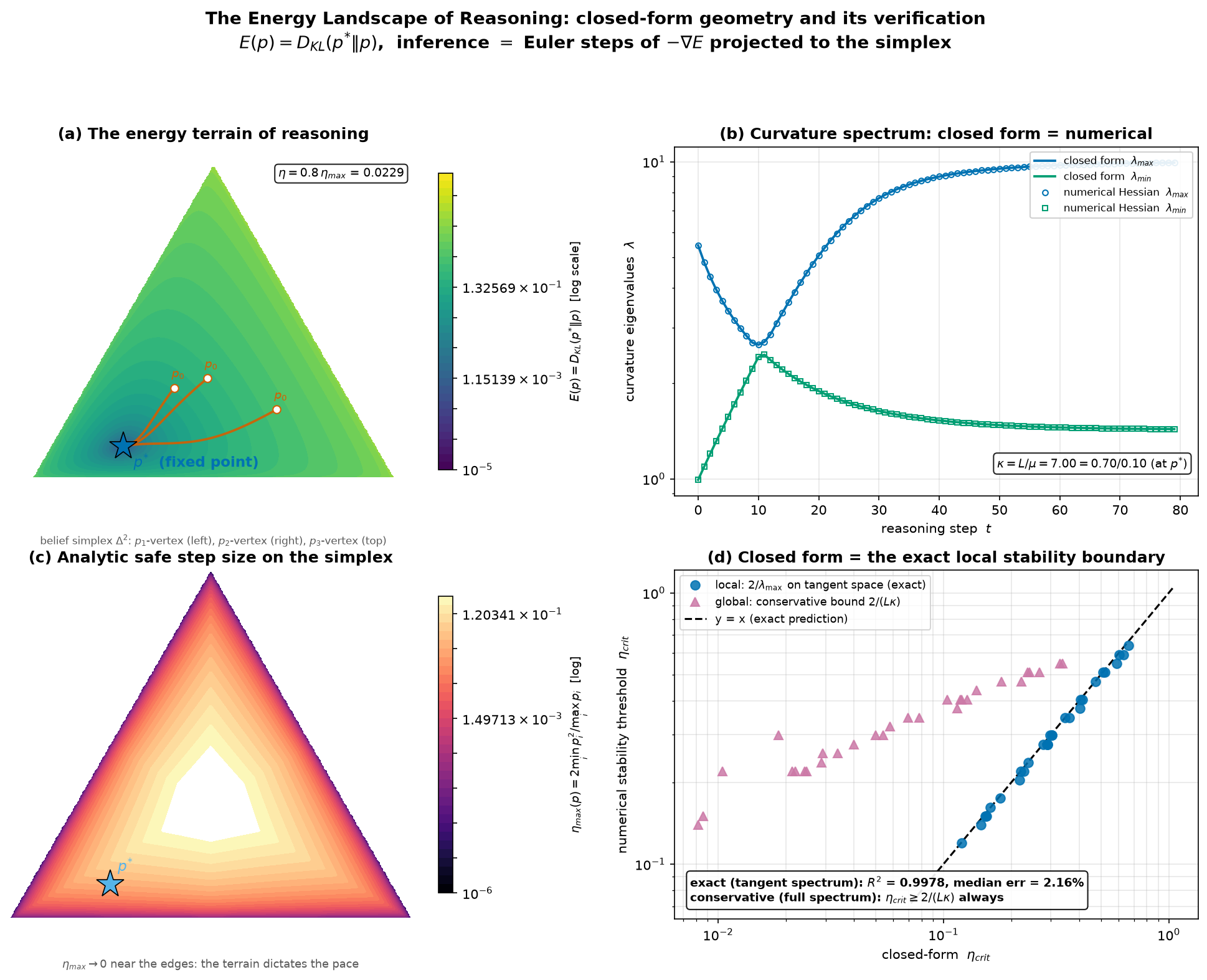
如何读图 1 的四个面板:
(a)地形存在。
(b)曲率谱:闭式 = 数值。 沿一条推理轨迹,解析谱(
(c)
(d)稳定边界:闭式精确预测数值。 局部扰动动力学的数值失稳阈值
这个实验顺带做了两处改进:
第一:精确的局部稳定界是切空间谱,不是全空间谱。 投影把动力学限制在切空间
的最大根。第 10 步的
第二:稳定性判据必须用渐近终点,而不是全程最大值。 动力学是否稳定,看的是
源码(完整可运行;运行时会把图保存为同目录下的 ch12_energy_terrain.png):
"""
Energy Landscape of Reasoning: Closed-Form Curvature and Safe Step Size
========================================================================

Demonstration accompanying the Yonglin Limit derivation.

Setup: belief simplex Delta^2 (3 classes). The reasoning energy is
    E(p) = D_KL(p* || p),  p* = target/attractor belief.
Inference = Euler steps of the gradient flow on E with projection to the
simplex:  p_{t+1} = proj_Delta(p_t - eta * grad E(p_t)).

Closed-form facts under study (true at the fixed point p = p*):
    Hess E(p)  = diag(q_i / p_i^2)   [general position; q_i = p*_i]
               -> diag(1/p_i)        [at p = p*]
    mu = lambda_min = 1/max_i p_i,  L = lambda_max = 1/min_i p_i
    kappa = L/mu = max_i p_i / min_i p_i          (spectral ratio / condition number)
    eta_max = 2 mu / L^2 = 2 / (L * kappa) = 2 min_i p_i^2 / max_i p_i

On the tangent space {v: sum v_i = 0} (the subspace preserved by the
projection) the exact local stability boundary is
    eta_crit = 2 / lambda_max,  lambda_max = largest eigenvalue of
    diag(1/q_i) restricted to the tangent space;
    for K = 3, lambda_max solves  3 q0 q1 q2 lam^2 - 2 (q0q1+q0q2+q1q2) lam + 1 = 0.
"""
import numpy as np
import matplotlib
matplotlib.use("Agg")
import matplotlib.pyplot as plt
from matplotlib.colors import LogNorm
from matplotlib.patheffects import withStroke

rng = np.random.default_rng(42)


# ----------------------------- core helpers -----------------------------
def proj_simplex(v):
    """Euclidean projection onto probability simplex (vectorized over last axis).
    Standard algorithm: find the last index j with u_j - (css_j - 1)/j > 0."""
    v = np.asarray(v, float)
    shape = v.shape
    v = v.reshape(-1, shape[-1])
    K = shape[-1]
    u = np.sort(v, axis=1)[:, ::-1]
    css = np.cumsum(u, axis=1)
    avg = (css - 1.0) / np.arange(1, K + 1)
    cond = u - avg > 0
    j = np.where(cond)[1]    # column indices of True entries (rows repeat)
    # last True index per row:
    last = np.array([np.where(cond[i])[0][-1] for i in range(len(cond))])
    theta = (css[np.arange(len(v)), last] - 1.0) / (last + 1)
    out = np.maximum(v - theta[:, None], 0.0)
    return out.reshape(shape)


def energy(p, pstar):
    """E(p) = D_KL(p* || p), elementwise-safe (p clipped away from 0)."""
    pc = np.clip(p, 1e-300, 1.0)
    with np.errstate(divide="ignore", invalid="ignore"):
        e = np.sum(pstar * np.log(pstar / pc), axis=-1)
    return np.where(np.all(p > 0, axis=-1), e, np.inf)


def grad_energy(p, pstar):
    return -pstar / np.clip(p, 1e-12, 1.0)


def euler_step(p, pstar, eta):
    return proj_simplex(p - eta * grad_energy(p, pstar))


def eta_max_closed(pstar):
    """Closed-form safe step size at the fixed point: 2 min^2 / max."""
    return 2.0 * np.min(pstar) ** 2 / np.max(pstar)


def hessian_numeric(p, pstar, eps=1e-6):
    """Central-difference Hessian of E at p (K=3)."""
    K = len(p)
    H = np.zeros((K, K))
    for i in range(K):
        for j in range(K):
            ei = np.zeros(K); ej = np.zeros(K)
            ei[i] = eps; ej[j] = eps
            H[i, j] = (energy(p + ei + ej, pstar) - energy(p + ei - ej, pstar)
                       - energy(p - ei + ej, pstar) + energy(p - ei - ej, pstar)) / (4 * eps * eps)
    return H


def to_xy(p):
    """Barycentric -> Cartesian (A=e1 at (0,0), B=e2 at (1,0), C=e3 at (0.5,sqrt3/2))."""
    return p[..., 1] * 1.0 + p[..., 2] * 0.5, p[..., 2] * (np.sqrt(3) / 2)


def from_xy(x, y):
    s = np.sqrt(3.0) / 2.0
    p3 = np.clip(y / s, 0.0, 1.0)
    p2 = np.clip(x - y / (np.sqrt(3.0)), 0.0, 1.0)
    p1 = 1.0 - p2 - p3
    mask = (p1 >= -1e-9) & (p2 >= -1e-9) & (p3 >= -1e-9)
    p1 = np.clip(p1, 0.0, 1.0)
    return np.stack([p1, p2, p3], axis=-1), mask


# ----------------------------- figure panels -----------------------------
PSTAR = np.array([0.70, 0.20, 0.10])
EMAX = eta_max_closed(PSTAR)          # ~ 2*0.01/0.7 = 0.02857
ETA_ILLUS = 0.8 * EMAX

fig, axes = plt.subplots(2, 2, figsize=(13.2, 10.4))
ps = withStroke(linewidth=3, foreground="white")

# ---------- (a) energy terrain + trajectories ----------
ax = axes[0, 0]
xgrid = np.linspace(-0.05, 1.05, 300)
ygrid = np.linspace(-0.05, np.sqrt(3) / 2 + 0.05, 260)
X, Y = np.meshgrid(xgrid, ygrid)
P, mask = from_xy(X, Y)
E = energy(P, PSTAR)
E = np.where(mask, E, np.nan)
lv = np.geomspace(1e-5, 50, 40)
cf = ax.contourf(X, Y, E, levels=lv, cmap="viridis", norm=LogNorm(vmin=1e-5, vmax=50))
cbar = fig.colorbar(cf, ax=ax, shrink=0.85)
cbar.set_label(r"$E(p)=D_{KL}(p^{*}\|p)$  [log scale]", fontsize=9)

starts = [np.array([1/3, 1/3, 1/3]), np.array([0.15, 0.60, 0.25]), np.array([0.45, 0.25, 0.30])]
for p0 in starts:
    p = p0.copy()
    xs, ys = [], []
    for t in range(120):
        p = euler_step(p, PSTAR, ETA_ILLUS)
        xs.append(to_xy(p)[0]); ys.append(to_xy(p)[1])
        if energy(p, PSTAR) < 1e-6:
            break
    ax.plot(xs, ys, lw=1.8, color="#D55E00", alpha=0.9)
    ax.plot(xs[0], ys[0], "o", ms=6, color="#D55E00", mfc="white")
    ax.annotate("$p_0$", (xs[0], ys[0]), textcoords="offset points", xytext=(-2, 8),
                fontsize=9, color="#D55E00")

px, py = to_xy(PSTAR)
ax.plot(px, py, "*", ms=22, color="#0072B2", mec="k", mew=0.8, zorder=10)
ax.annotate(r"$p^{*}$  (fixed point)", (px, py), textcoords="offset points",
            xytext=(8, -16), fontsize=11, color="#0072B2", fontweight="bold")
ax.text(0.98, 0.94, f"$\\eta=0.8\\,\\eta_{{max}}$ = {ETA_ILLUS:.4f}",
        transform=ax.transAxes, ha="right", va="top", fontsize=9,
        bbox=dict(boxstyle="round,pad=0.3", fc="white", alpha=0.85))
ax.set_title("(a) The energy terrain of reasoning", fontsize=12, fontweight="bold")
ax.text(0.5, -0.14, "belief simplex $\\Delta^2$: $p_1$-vertex (left), $p_2$-vertex (right), $p_3$-vertex (top)",
        transform=ax.transAxes, ha="center", fontsize=8, color="0.35")
ax.set_aspect("equal"); ax.axis("off")

# ---------- (b) curvature spectrum along one trajectory ----------
ax = axes[0, 1]
p = np.array([1/3, 1/3, 1/3])
lmax_a, lmin_a, kap_a = [], [], []
lmax_n, lmin_n = [], []
p_rec = []
for t in range(80):
    p = euler_step(p, PSTAR, ETA_ILLUS)
    p_rec.append(p.copy())
for p in p_rec:
    lmax_a.append(np.max(PSTAR / p**2)); lmin_a.append(np.min(PSTAR / p**2))
    H = hessian_numeric(p, PSTAR)
    w = np.linalg.eigvalsh(H)
    lmax_n.append(w[-1]); lmin_n.append(w[0])
ts = np.arange(len(p_rec))
ax.plot(ts, lmax_a, color="#0072B2", lw=1.8, label=r"closed form  $\lambda_{max}$")
ax.plot(ts, lmin_a, color="#009E73", lw=1.8, label=r"closed form  $\lambda_{min}$")
ax.plot(ts, lmax_n, "o", ms=4.2, color="#0072B2", mfc="none", label=r"numerical Hessian  $\lambda_{max}$")
ax.plot(ts, lmin_n, "s", ms=4.2, color="#009E73", mfc="none", label=r"numerical Hessian  $\lambda_{min}$")
ax.set_yscale("log")
ax.set_xlabel("reasoning step  $t$", fontsize=10)
ax.set_ylabel("curvature eigenvalues  $\\lambda$", fontsize=10)
ax.set_title("(b) Curvature spectrum: closed form = numerical", fontsize=12, fontweight="bold")
ax.legend(fontsize=8, framealpha=0.9, loc="upper right")
ax.grid(alpha=0.3)
kap = PSTAR.max() / PSTAR.min()
ax.text(0.98, 0.08, r"$\kappa = L/\mu = %.2f = 0.70/0.10$ (at $p^{*}$)" % kap,
        transform=ax.transAxes, ha="right", fontsize=9,
        bbox=dict(boxstyle="round,pad=0.3", fc="white", alpha=0.85))

# ---------- (c) analytic eta_max surface ----------
ax = axes[1, 0]
XS, YS = np.meshgrid(np.linspace(0, 1, 260), np.linspace(0, np.sqrt(3) / 2, 230))
PS, maskC = from_xy(XS, YS)
eta = np.where(maskC & np.all(PS > 1e-4, axis=-1),
               2.0 * np.min(PS, axis=-1) ** 2 / np.max(PS, axis=-1), np.nan)
eta = np.where(maskC, eta, np.nan)
lv2 = np.geomspace(1e-6, 0.25, 35)
cf2 = ax.contourf(XS, YS, eta, levels=lv2, cmap="magma", norm=LogNorm(vmin=1e-6, vmax=0.25))
cbar2 = fig.colorbar(cf2, ax=ax, shrink=0.85)
cbar2.set_label(r"$\eta_{max}(p)=2\min_i p_i^2/\max_i p_i$  [log]", fontsize=9)
ax.plot(px, py, "*", ms=22, color="#56B4E9", mec="k", mew=0.8, zorder=10)
ax.annotate(r"$p^{*}$", (px, py), textcoords="offset points", xytext=(6, 10),
            fontsize=11, color="#56B4E9", fontweight="bold")
ax.set_title("(c) Analytic safe step size on the simplex", fontsize=12, fontweight="bold")
ax.text(0.5, -0.14, "$\\eta_{max} \\to 0$ near the edges: the terrain dictates the pace",
        transform=ax.transAxes, ha="center", fontsize=8.5, color="0.35")
ax.set_aspect("equal"); ax.axis("off")

# ---------- (d) closed form vs numerical stability boundary ----------
ax = axes[1, 1]


def lambda_max_tangent(q):
    """Largest eigenvalue of diag(q_i^{-1}) restricted to the tangent space {v: sum v_i = 0}.
    K = 3: analytic root of  3 q0 q1 q2 lam^2 - 2 (q0q1+q0q2+q1q2) lam + 1 = 0."""
    q0, q1, q2 = q
    a = 3 * q0 * q1 * q2
    b = -2 * (q0 * q1 + q0 * q2 + q1 * q2)
    c = 1.0
    disc = b * b - 4 * a * c
    lam = (-b + np.sqrt(disc)) / (2 * a)
    return lam


def eta_crit_tangent_closed(q):
    """Exact local stability boundary: eta_safe < 2 / lambda_max of Hessian on the tangent space."""
    return 2.0 / lambda_max_tangent(q)


# ---------- (d) closed form vs numerical stability boundary ----------
ax = axes[1, 1]

etas_scan = np.logspace(-4.0, 0.6, 140)

# --- LOCAL analysis: perturbations of p*; exact prediction = tangent-space spectrum ---
local_ana, local_num = [], []
for _ in range(30):
    ps_ = rng.dirichlet(np.ones(3)) * 0.9 + 0.05
    ps_ = ps_ / ps_.sum()
    pert = [proj_simplex(ps_ + 0.02 * rng.normal(0, 1, 3) * np.array([1, 0.5, 0.25])) for _ in range(8)]
    # asymptotic stability: final distance does not grow
    worst = np.zeros(len(etas_scan))
    for p0 in pert:
        P = np.broadcast_to(p0.copy(), (len(etas_scan), 3)).copy()
        d0 = np.linalg.norm(p0 - ps_)
        for _ in range(500):
            P = proj_simplex(P - etas_scan[:, None] * (-ps_ / np.clip(P, 1e-12, 1.0)))
        worst = np.maximum(worst, np.linalg.norm(P - ps_, axis=1) / d0)
    idx = np.where(worst < 1.0)[0]
    local_num.append(etas_scan[idx[-1]] if len(idx) else etas_scan[0] / 2)
    local_ana.append(eta_crit_tangent_closed(ps_))

# --- GLOBAL analysis: from uniform prior; conservative closed form = full-space spectrum ---
glob_ana, glob_num = [], []
for _ in range(30):
    ps_ = rng.dirichlet(np.ones(3)) * 0.9 + 0.05
    ps_ = ps_ / ps_.sum()
    P = np.broadcast_to(np.full(3, 1 / 3), (len(etas_scan), 3)).copy()
    for _ in range(400):
        P = proj_simplex(P - etas_scan[:, None] * (-ps_ / np.clip(P, 1e-12, 1.0)))
    fk = np.sum(ps_ * np.log(np.clip(ps_, 1e-12, 1) / np.clip(P, 1e-12, 1)), axis=1)
    idx = np.where(fk < 1e-3)[0]
    glob_num.append(etas_scan[idx[-1]] if len(idx) else etas_scan[0] / 2)
    glob_ana.append(eta_max_closed(ps_))

local_ana, local_num = np.array(local_ana), np.array(local_num)
glob_ana, glob_num = np.array(glob_ana), np.array(glob_num)

ax.loglog(local_ana, local_num, "o", ms=7, color="#0072B2", alpha=0.85, zorder=6,
          label=r"local: $2/\lambda_{\max}$ on tangent space (exact)")
ax.loglog(glob_ana, glob_num, "^", ms=7, color="#CC79A7", alpha=0.85, zorder=5,
          label=r"global: conservative bound $2/(L\kappa)$")
lims = [min(local_ana.min(), local_num.min()) * 0.6, max(local_ana.max(), local_num.max()) * 1.6]
ax.loglog(lims, lims, "k--", lw=1.5, label="y = x (exact prediction)")
logR = np.corrcoef(np.log10(local_ana), np.log10(local_num))[0, 1] ** 2
med = np.median(np.abs(local_num - local_ana) / local_ana)
ax.set_xlabel(r"closed-form  $\eta_{crit}$", fontsize=10)
ax.set_ylabel("numerical stability threshold  $\\eta_{crit}$", fontsize=10)
ax.set_title("(d) Closed form = the exact local stability boundary", fontsize=12, fontweight="bold")
ax.legend(fontsize=8.5, loc="upper left")
ax.grid(alpha=0.3, which="both")
ax.text(0.03, 0.05, f"exact (tangent spectrum): $R^2$ = {logR:.4f}, median err = {med:.2%}\nconservative (full spectrum): $\\eta_{{crit}} \\geq 2/(L\\kappa)$ always",
        transform=ax.transAxes, fontsize=9, color="k", fontweight="bold",
        bbox=dict(boxstyle="round,pad=0.3", fc="white", alpha=0.9))

fig.suptitle("The Energy Landscape of Reasoning: closed-form geometry and its verification\n"
             r"$E(p)=D_{KL}(p^{*}\|p)$,  inference $=$ Euler steps of $-\nabla E$ projected to the simplex",
             fontsize=13.5, fontweight="bold", y=0.995)
fig.tight_layout(rect=[0, 0, 1, 0.95])
out = "ch12_energy_terrain.png"   # saves next to the script
fig.savefig(out, dpi=150, bbox_inches="tight")
print("saved:", out)
print(f"eta_max closed form (p* = {PSTAR}): {EMAX:.6f}")
print(f"kappa at fixed point: {PSTAR.max()/PSTAR.min():.2f}")
print(f"panel d: local R^2(log-log) = {logR:.4f}, n = {len(local_ana)}, median err = {med:.2%}")
print(f"panel d: global: numerically stable region >= eta_max (projection adds stability)")
图 1 与源码:李籽溪(兔狲教授),2026。实验脚本 ch12_energy_terrain.py(完整代码见本节代码块)。
10.1 真实 LLM 上的直接证据:信念锚点、证据强度与记忆衰减
上一节的数值实验验证了公式的内部自洽性:动力学本来就是按闭式解的欧拉步构造的,当然会跟着它走。本节给出真实 LLM 上的直接证据:用真实模型(DeepSeek-V4-flash,reasoning 类型)实例化第七节的推断算子 ch12_llm_evidence.png;实验的完整数据设计如下(实验本身与数字都活在图中——涉及真实模型 API 的脚本不在此重复)。
实验设置。 三色球袋世界,仍在信念单纯形
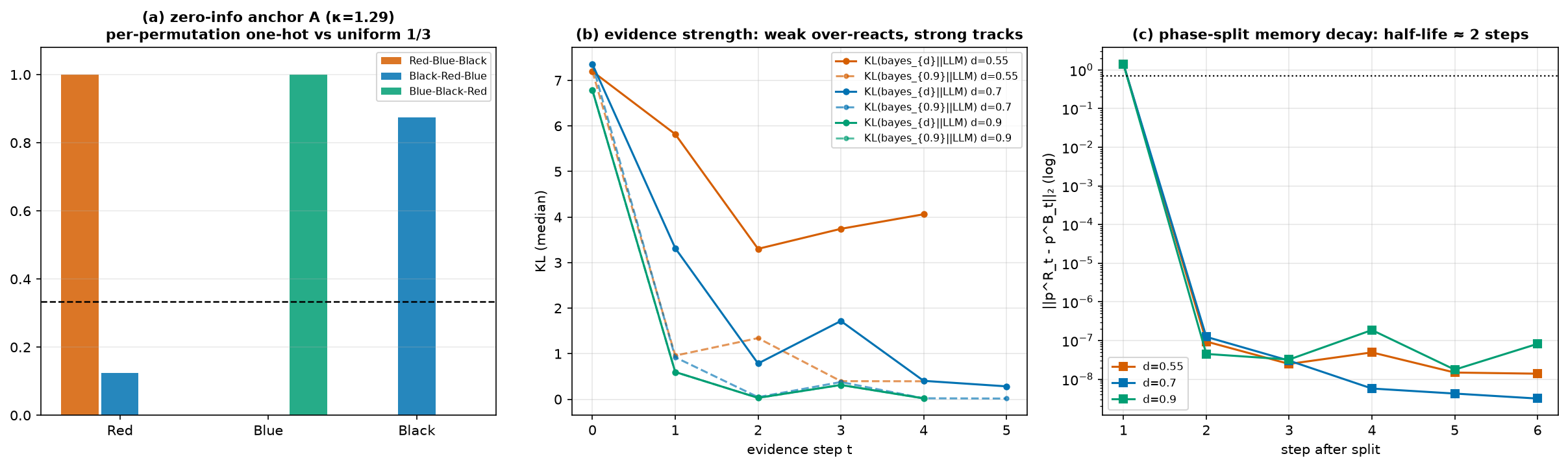
如何读图 12.2 的三个面板——(a)锚点:三种选项排列下的零信息信念都贴近某个顶点(位置偏置),全局平均
结果 1:零信息锚点
结果 2:输出层信念是尖峰的——推理贴着单纯形边界走。 在第 0 步(提示词已写明球袋比例 7/2/1,还没有报告),中位
结果 3:证据强度吸收是不对称的——弱证据被放大,强证据被忠实跟随。 下表(中位 KL:LLM 信念与真实后验的 KL / 与
| d | t=1 | t=2 | t=3 | t=4 | t=5 |
|---|---|---|---|---|---|
| 0.55(真实后验 / | 5.82 / 0.96 | 3.30 / 1.34 | 3.74 / 0.40 | 4.06 / 0.40 | — |
| 0.70 | 3.32 / 0.92 | 0.79 / 0.05 | 1.72 / 0.38 | 0.40 / 0.02 | 0.28 / 0.02 |
| 0.90 | 0.60 | 0.03 | 0.31 | 0.02 | — |
对
结果 4:压缩与记忆——相位差半衰期约 2 步。 同一个世界,同一串报告尾部(第 2–6 条报告相同);两条轨迹唯一的区别是第一条报告是红还是蓝。初始分叉距离
对理论四行交叉核对:锚点 = 第 9 步先验锚点
图 12.2 与源码:李籽溪(兔狲教授),2026。实验见 10.1 节(脚本的 API 版本不在书中展开)。
10.2 同一极限,在一台笔记本上:一幅你自己能画的蛛网图
10.1 节测量了大型闭参数模型的信念动力学。那个实验的代价是:读者拿到的是数字,不是实验。本小节把同一个极限做成你能在自己笔记本上跑的形式。模型是 GPT-2,约 1.24 亿参数,开源且小;信念是一维的;得到的图是离散动力系统(第七节,迭代序列
实验设置。 24 个传递链问题(例如“A 比 B 高。B 比 C 高。A 比 C 高吗?”)。它们全部为真,所以真实答案分布恰好是
结果 1:锚点是测出来的,不是假设的。 24 个问题上的初始信念均值为 0.4045;逐个问题的值在 0.1993 到 0.7105 之间。一段文本的先验锚点是文本的函数:road/path/lane 链条上模型从 0.199 起步,X/Y/Z 链条上从 0.710 起步。一个问题背后没有单一的“训练数据边缘分布”:先验锚点是逐问题锚点的混合物。
结果 2:测得的映射是平的——一步,不是阶梯。 整个网格上,
结果 3:有效推理窗口是一步。 在 128 步 rollout 中,中位
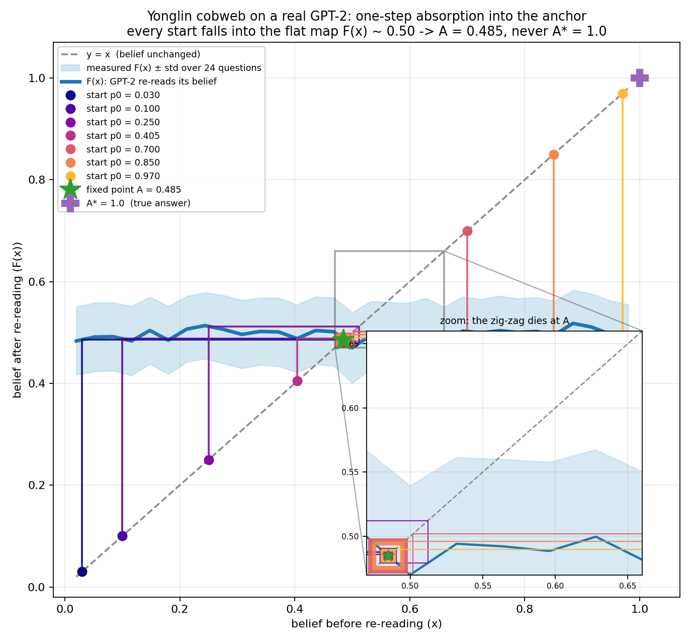
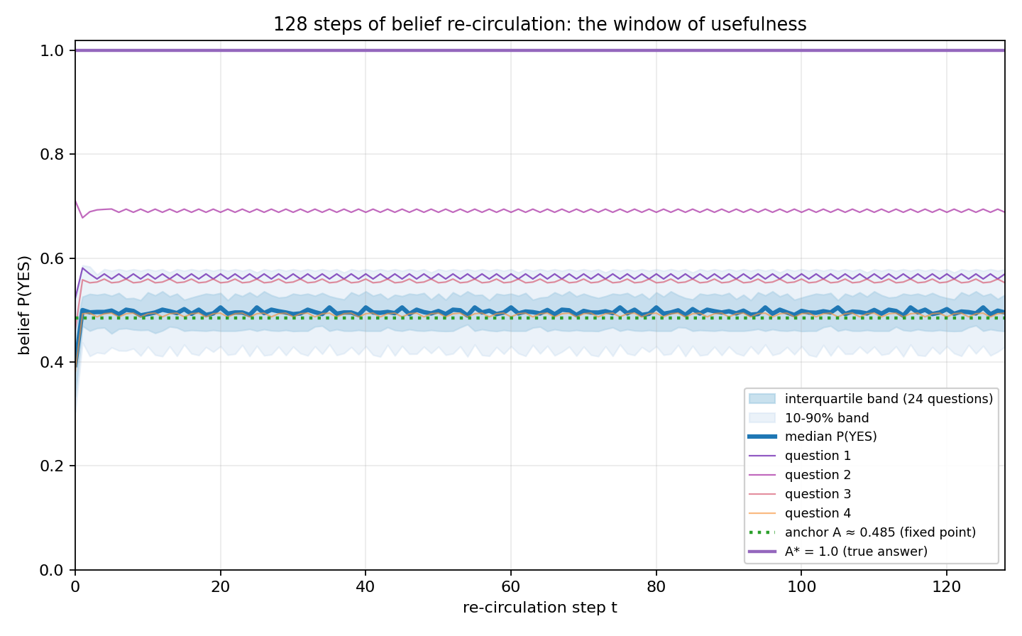
如何读图 12.3(蛛网图)。 灰色虚线对角线是“信念不变”:线上的任何点都是候选不动点。蓝线是测得的映射
如何读图 12.4(时间序列)。 每条线是一个问题在 128 步上的信念;阴影带是 24 个问题的四分位带与 10–90 百分位带。看
一个诚实的保留。这里的信念是一个 1.24 亿参数状态的一维投影,而把数字写回提示词是“把信念写下来”的一种风格化做法。这个实验展示的不是 GPT-2 的心理,而是这个投影的动力学:平坦的映射、位于先验的锚点、一步的窗口。它毫无建模地表明:在真实模型上,永霖极限不是缓慢的淡出——是悬崖。
动手玩。 改问题库,改注入置信度的模板,运行 --model gpt2-medium,改 --grid 和 --steps。锚点会动(它总会动);映射保持平坦;
源码(完整可运行;保存为 yonglin_gpt2.py 后运行。它会在自身旁边保存两张 PNG:yonglin_cobweb_measured.png = 图 12.3,yonglin_belief_evolution.png = 图 12.4):
#!/usr/bin/env python3
"""
Yonglin Cobweb: Belief-Recirculation Dynamics on a Real GPT-2
==============================================================
Companion experiment for The Reasoning Kingdom, Chapter 12
(Sections 5, 7, 10.1 and 10.2).

THE IDEA IN ONE PARAGRAPH
-------------------------
Yonglin's formula says: belief dynamics p_{t+1} = F(p_t) converges to the
prior anchor A, not to the true answer A* (A != A*). Section 10.1 verifies anchors and evidence
absorption on a large closed API model, but the reader cannot run it.
Section 10.2 gives the version you can RUN and PLAY WITH: a small open
model (GPT-2, ~124M params, runs on a laptop), a one-dimensional belief
state P(YES), and the belief recirculated through the model itself.
Each step you read the model's belief from its next-token logits, write
that belief back into the prompt as text, and measure the next belief.
That defines a one-dimensional dynamical system p_{t+1} = F(p_t) that you
can measure, plot, and look at as a COBWEB picture: the curve y = F(x),
the diagonal y = x, and the zig-zag staircase of the iterated belief.

WHAT THE SCRIPT DOES
--------------------
  1. loads the model (default: gpt2; check the HuggingFace cache first).
  2. read_belief(prompt): P(YES) = sigmoid(logit_YES - logit_NO).
  3. measure_F(): 31 grid points x in [0, 1], the belief written back
     into the prompt; F measured over 24 questions.
  4. rollouts(): 128 steps of belief re-circulation from each question's
     natural start; prints summaries and the distribution over questions.
  5. cobweb_points(): the classic zig-zag construction.
  6. two figures:
       (a) yonglin_cobweb_measured.png       -- the cobweb itself
       (b) yonglin_belief_evolution.png      -- p_t vs t, all 128 steps

HONESTY CAVEATS
---------------
  * "Belief" is a one-dimensional projection (next-token softmax of
    YES/NO). The real state is 124M-dimensional; this is the deliberate
    cut that makes the cobweb picture possible.
  * Writing the number p back into the prompt is a stylized way of
    writing the belief down. The model re-reads a text that contains
    its own last belief; it does not literally iterate a hidden state.
  * Every number printed and every point plotted comes from a live run
    of the model on this machine. Nothing is scripted.

Run:  python3 yonglin_gpt2.py
      python3 yonglin_gpt2.py --model gpt2-medium --steps 128 --grid 31
"""
import argparse
import os
from pathlib import Path

import matplotlib
matplotlib.use("Agg")
import matplotlib.pyplot as plt
import numpy as np
import torch
from transformers import GPT2LMHeadModel, GPT2Tokenizer

# ---------------------------------------------------------------------------
# 0. The question bank (24 short transitive-chain questions, all TRUE)
# ---------------------------------------------------------------------------
QUESTIONS = [
    "A is taller than B. B is taller than C. Is A taller than C?",
    "X is larger than Y. Y is larger than Z. Is X larger than Z?",
    "P is heavier than Q. Q is heavier than R. Is P heavier than R?",
    "The oak is older than the birch. The birch is older than the elm. Is the oak older than the elm?",
    "K is faster than L. L is faster than M. Is K faster than M?",
    "The river is longer than the stream. The stream is longer than the brook. Is the river longer than the brook?",
    "Red is darker than pink. Pink is darker than cream. Is red darker than cream?",
    "The mountain is steeper than the hill. The hill is steeper than the slope. Is the mountain steeper than the slope?",
    "Steel is harder than iron. Iron is harder than tin. Is steel harder than tin?",
    "The tiger is stronger than the wolf. The wolf is stronger than the fox. Is the tiger stronger than the fox?",
    "The poem is longer than the song. The song is longer than the haiku. Is the poem longer than the haiku?",
    "Bob is faster than Anne. Anne is faster than Carl. Is Bob faster than Carl?",
    "Winter is colder than autumn. Autumn is colder than spring. Is winter colder than spring?",
    "Silver is shinier than copper. Copper is shinier than iron. Is silver shinier than iron?",
    "The soup is hotter than the stew. The stew is hotter than the porridge. Is the soup hotter than the porridge?",
    "The whale is larger than the elephant. The elephant is larger than the horse. Is the whale larger than the horse?",
    "The road is longer than the path. The path is longer than the lane. Is the road longer than the lane?",
    "The clock is older than the watch. The watch is older than the phone. Is the clock older than the phone?",
    "Sarah is taller than Kate. Kate is taller than Anna. Is Sarah taller than Anna?",
    "The ocean is deeper than the lake. The lake is deeper than the pond. Is the ocean deeper than the pond?",
    "The horse is faster than the dog. The dog is faster than the cat. Is the horse faster than the cat?",
    "The house is taller than the garage. The garage is taller than the shed. Is the house taller than the shed?",
    "The sun is hotter than the flame. The flame is hotter than the candle. Is the sun hotter than the candle?",
    "Matthew is slower than Helen. Helen is slower than George. Is Matthew slower than George?",
]
ANSWER = "YES"                      # every question above is TRUE (A* = 1.0)
ID_YES, ID_NO = None, None          # filled in main()
TEMPLATE_ANSWER = "\nAnswer with exactly one word: YES or NO."


def confidence_template(p: float) -> str:
    """Write the current belief back into the prompt as one line."""
    return f"\nConfidence so far: P(YES) = {p:.3f}."


# ---------------------------------------------------------------------------
# 1. Belief reader
# ---------------------------------------------------------------------------
@torch.no_grad()
def read_belief(model, tokenizer, prompt: str, device) -> float:
    """P(YES) = sigmoid(logit_YES - logit_NO) at the last position."""
    input_ids = tokenizer(prompt, return_tensors="pt").input_ids.to(device)
    logits = model(input_ids).logits[0, -1]
    return float(torch.sigmoid(logits[ID_YES] - logits[ID_NO]).item())


def ask(model, tokenizer, question: str, p: float, device) -> float:
    """One application of the map: belief p in, belief F(p) out."""
    prompt = question + confidence_template(p) + TEMPLATE_ANSWER
    return read_belief(model, tokenizer, prompt, device)


# ---------------------------------------------------------------------------
# 2. Measuring F on a grid
# ---------------------------------------------------------------------------
def measure_F(model, tokenizer, questions, grid_n: int, device):
    """F(x) on a grid, averaged over questions: (xs, mean, std)."""
    xs = np.linspace(0.02, 0.98, grid_n)
    Fs = np.zeros((len(questions), grid_n))
    for qi, q in enumerate(questions):
        for xi, x in enumerate(xs):
            Fs[qi, xi] = ask(model, tokenizer, q, float(x), device)
    return xs, Fs.mean(axis=0), Fs.std(axis=0)


# ---------------------------------------------------------------------------
# 3. Rollouts
# ---------------------------------------------------------------------------
def rollouts(model, tokenizer, questions, steps: int, device):
    """p_0 = natural belief; p_{t+1} = F(p_t). Returns array (Q, steps+1)."""
    traj = np.zeros((len(questions), steps + 1))
    for qi, q in enumerate(questions):
        p0 = read_belief(model, tokenizer, q + TEMPLATE_ANSWER, device)
        traj[qi, 0] = p0
        for t in range(steps):
            traj[qi, t + 1] = ask(model, tokenizer, q, float(traj[qi, t]), device)
    return traj


# ---------------------------------------------------------------------------
# 5. Cobweb construction
# ---------------------------------------------------------------------------
def cobweb_points(fn, p0, steps: int):
    """The zig-zag: vertical to the curve, horizontal to the diagonal."""
    pts_x, pts_y = [p0], [p0]
    p = p0
    for _ in range(steps):
        f = float(np.asarray(fn(np.array([p])))[0])
        pts_x.append(p)
        pts_y.append(f)
        p = f
        pts_x.append(p)
        pts_y.append(p)
    return np.array(pts_x), np.array(pts_y)


def interpolate_F(xs, Fm):
    def fn(x):
        return np.interp(np.asarray(x, dtype=float), xs, Fm)
    return fn


def fixed_point(xs, Fm):
    """Root of F(x) - x by linear interpolation on the grid."""
    g = Fm - xs
    idx = np.where(np.diff(np.sign(g)) != 0)[0]
    if not len(idx):
        return None
    i = idx[0]
    return float(xs[i] - g[i] * (xs[i + 1] - xs[i]) / (g[i + 1] - g[i]))


# ---------------------------------------------------------------------------
# 6. Figures
# ---------------------------------------------------------------------------
def plot_measured_cobweb(xs, Fm, Fs, p0_mean, fixed, out_dir):
    """(a) The cobweb itself: multi-start, the flat anchor map."""
    fig, ax = plt.subplots(figsize=(8.6, 8.0))
    ax.plot(xs, xs, color="0.55", lw=1.6, ls="--", label="y = x  (belief unchanged)")
    ax.fill_between(xs, Fm - Fs, Fm + Fs, color="#9ecae1", alpha=0.45,
                    label="measured F(x) ± std over 24 questions")
    ax.plot(xs, Fm, color="#1f77b4", lw=3.2, label="F(x): GPT-2 re-reads its belief")
    starts = [0.03, 0.10, 0.25, float(p0_mean), 0.70, 0.85, 0.97]
    fn = interpolate_F(xs, Fm)
    colors = plt.cm.plasma(np.linspace(0, 0.85, len(starts)))
    for c, p0 in zip(colors, starts):
        px, py = cobweb_points(fn, float(p0), 20)
        ax.plot(px, py, color=c, lw=1.7, alpha=0.9)
        ax.plot([p0], [p0], "o", ms=8, color=c, zorder=6, label=f"start p0 = {p0:.3f}")
    ax.plot(fixed, fixed, "*", color="#2ca02c", ms=20, zorder=7,
            label=f"fixed point A = {fixed:.3f}")
    ax.plot([1.0], [1.0], "P", color="#9467bd", ms=15, zorder=7,
            label="A* = 1.0  (true answer)")
    ax.set_xlim(-0.02, 1.07); ax.set_ylim(-0.02, 1.07)
    ax.set_xlabel("belief before re-reading (x)")
    ax.set_ylabel("belief after re-reading (F(x))")
    ax.set_title("Yonglin cobweb on a real GPT-2: one-step absorption into the anchor\n"
                 f"every start falls into the flat map F(x) ~ {np.mean(Fm):.2f} "
                 f"-> A = {fixed:.3f}, never A* = 1.0",
                 fontsize=11.5)
    ax.legend(loc="upper left", fontsize=8.0, framealpha=0.92)
    ax.grid(alpha=0.25)
    axin = ax.inset_axes([0.50, 0.04, 0.44, 0.44])
    axin.plot(xs, xs, color="0.55", lw=1.2, ls="--")
    axin.plot(xs, Fm, color="#1f77b4", lw=2.0)
    axin.fill_between(xs, Fm - Fs, Fm + Fs, color="#9ecae1", alpha=0.4)
    for c, p0 in zip(colors, starts):
        px, py = cobweb_points(fn, float(p0), 20)
        axin.plot(px, py, color=c, lw=1.0, alpha=0.9)
    axin.plot([fixed], [fixed], "*", color="#2ca02c", ms=11)
    axin.set_xlim(0.47, 0.66); axin.set_ylim(0.47, 0.66)
    axin.set_xticks([0.50, 0.55, 0.60, 0.65]); axin.set_yticks([0.50, 0.55, 0.60, 0.65])
    axin.tick_params(labelsize=7)
    axin.set_title("zoom: the zig-zag dies at A", fontsize=8.5)
    axin.grid(alpha=0.3)
    # the frame that tells the reader WHICH region of the main plot is zoomed:
    ax.indicate_inset_zoom(axin, edgecolor="0.30", lw=1.6)
    fig.tight_layout()
    path = os.path.join(out_dir, "yonglin_cobweb_measured.png")
    fig.savefig(path, dpi=160)
    plt.close(fig)
    return path


def plot_evolution(traj, fixed, out_dir):
    """(b) p_t vs t over 128 steps: median, quartile band, samples."""
    fig, ax = plt.subplots(figsize=(9.0, 5.6))
    t = np.arange(traj.shape[1])
    med = np.median(traj, axis=0)
    q1, q3 = np.percentile(traj, [25, 75], axis=0)
    lo, hi = np.percentile(traj, [10, 90], axis=0)
    ax.fill_between(t, q1, q3, color="#9ecae1", alpha=0.55,
                    label="interquartile band (24 questions)")
    ax.fill_between(t, lo, hi, color="#c6dbef", alpha=0.35,
                    label="10-90% band")
    ax.plot(t, med, color="#1f77b4", lw=2.8, label="median P(YES)")
    for qi in range(min(4, traj.shape[0])):
        ax.plot(t, traj[qi], color=plt.cm.plasma(0.15 + 0.2 * qi),
                lw=1.0, alpha=0.65, label=f"question {qi + 1}")
    ax.axhline(fixed, color="#2ca02c", ls=":", lw=2.0,
               label=f"anchor A ≈ {fixed:.3f} (fixed point)")
    ax.axhline(1.0, color="#9467bd", ls="-", lw=2.0, label="A* = 1.0 (true answer)")
    ax.set_xlim(0, traj.shape[1] - 1)
    ax.set_ylim(0.0, 1.02)
    ax.set_xlabel("re-circulation step t")
    ax.set_ylabel("belief P(YES)")
    ax.set_title("128 steps of belief re-circulation: the window of usefulness",
                 fontsize=11.5)
    ax.legend(loc="lower right", fontsize=8.0, framealpha=0.92)
    ax.grid(alpha=0.25)
    fig.tight_layout()
    path = os.path.join(out_dir, "yonglin_belief_evolution.png")
    fig.savefig(path, dpi=160)
    plt.close(fig)
    return path


# ---------------------------------------------------------------------------
def main():
    ap = argparse.ArgumentParser(description="Yonglin cobweb experiment on GPT-2")
    ap.add_argument("--model", default="gpt2")
    ap.add_argument("--steps", type=int, default=128)
    ap.add_argument("--grid", type=int, default=31)
    ap.add_argument("--out", default=os.path.dirname(os.path.abspath(__file__)))
    ap.add_argument("--replot", action="store_true",
                    help="skip measurement, redraw figures from the cached data")
    args = ap.parse_args()
    out_dir = args.out
    Path(out_dir).mkdir(parents=True, exist_ok=True)
    cache_path = os.path.join(out_dir, "yonglin_cache.npz")
    if args.replot and os.path.exists(cache_path):
        data = np.load(cache_path)
        xs, Fm, Fs, traj, p0s = (data["xs"], data["Fm"], data["Fs"],
                                 data["traj"], data["p0s"])
        p0_mean = float(np.mean(p0s))
        print(f"[replot] loaded cached data from {cache_path}")
    else:
        device = "mps" if torch.backends.mps.is_available() else "cpu"
        print(f"[setup] model={args.model} device={device}")
        tokenizer = GPT2Tokenizer.from_pretrained(args.model)
        model = GPT2LMHeadModel.from_pretrained(args.model).to(device).eval()
        global ID_YES, ID_NO
        ID_YES = tokenizer.encode(" YES")[0]
        ID_NO = tokenizer.encode(" NO")[0]
        print(f"[setup] YES token={ID_YES}  NO token={ID_NO}")
        print(f"\n[1] Initial belief per question (no confidence injected):")
        p0s = []
        for q in QUESTIONS:
            p0 = read_belief(model, tokenizer, q + TEMPLATE_ANSWER, device)
            p0s.append(p0)
            print(f"    P(YES) = {p0:.4f}   | {q[:62]}")
        p0_mean = float(np.mean(p0s))
        print(f"    mean p0 = {p0_mean:.4f}   (the measured prior anchor A)")
        print(f"\n[2] Measuring F on {args.grid} grid points x {len(QUESTIONS)} questions ...")
        xs, Fm, Fs = measure_F(model, tokenizer, QUESTIONS, args.grid, device)
        for x, fm, fs in zip(xs, Fm, Fs):
            print(f"    x={x:.3f}   F_mean={fm:.4f}   F_std={fs:.4f}")
        print(f"\n[3] Rollouts ({args.steps} steps of belief re-circulation):")
        traj = rollouts(model, tokenizer, QUESTIONS, args.steps, device)
        for t in range(0, args.steps + 1, 16):
            row = traj[:, t]
            print(f"    t={t:3d}  median={np.median(row):.4f}  "
                  f"q1={np.percentile(row, 25):.4f} q3={np.percentile(row, 75):.4f}  "
                  f"min={row.min():.4f}  max={row.max():.4f}")
        np.savez_compressed(cache_path, xs=xs, Fm=Fm, Fs=Fs, traj=traj,
                            p0s=np.asarray(p0s, dtype=float))
        print(f"\n[cache] saved measured data to {cache_path}")
    fixed = fixed_point(xs, Fm)
    print(f"\n[4] Fixed point of the measured map: A = {fixed:.4f}")
    print(f"    True answer A* = 1.0.  Gap = {abs(fixed - 1.0):.4f}")
    print(f"\n[5] Final belief after {args.steps} steps: "
          f"median={np.median(traj[:, -1]):.4f}")
    print(f"    One-step view: p0 mean={p0_mean:.4f}, p1 median={np.median(traj[:, 1]):.4f}")
    p1 = plot_measured_cobweb(xs, Fm, Fs, p0_mean, fixed, out_dir)
    p2 = plot_evolution(traj, fixed, out_dir)
    print(f"\n[6] Figures written:")
    for p in (p1, p2):
        print(f"    {p}")
    print("\nDone. The zig-zag in the first figure is Yonglin's formula,\n"
          "drawn from a real model instead of a formula.")


if __name__ == "__main__":
    main()
运行脚本,你会看到(真实运行的节选——下面的数字正是由这份脚本、在 macOS MPS 设备上的 gpt2 产生的;尾部是这次运行的代表性输出):
[setup] model=gpt2 device=mps
[setup] YES token=21560  NO token=8005
[1] Initial belief per question (no confidence injected):
    P(YES) = 0.5230   | A is taller than B. B is taller than C. Is A taller than C?
    P(YES) = 0.7105   | X is larger than Y. Y is larger than Z. Is X larger than Z?
    P(YES) = 0.4635   | P is heavier than Q. Q is heavier than R. Is P heavier than R?
    P(YES) = 0.1993   | The road is longer than the path. The path is longer than the lane. Is the road longer than the lane?
    P(YES) = 0.3056   | The tiger is stronger than the wolf. The wolf is stronger than the fox. Is the tiger stronger than the fox?
    P(YES) = 0.4031   | Winter is colder than autumn. Autumn is colder than spring. Is winter colder than spring?
    ...
    mean p0 = 0.4045   (the measured prior anchor A)
[2] Measuring F on 31 grid points x 24 questions ...
    x=0.020   F_mean=0.4834   F_std=0.0668
    x=0.212   F_mean=0.5067   F_std=0.0647
    x=0.500   F_mean=0.4700   F_std=0.0693
    x=0.788   F_mean=0.5002   F_std=0.0666
    x=0.980   F_mean=0.4867   F_std=0.0681
[3] Rollouts (128 steps of belief re-circulation):
    t=  0  median=0.3944  q1=0.3338  q3=0.4611  min=0.1993  max=0.7105
    t= 16  median=0.4930  q1=0.4615  q3=0.5241  min=0.3800  max=0.6885
    t= 32  median=0.5009  q1=0.4601  q3=0.5316  min=0.3800  max=0.6885
    t= 64  median=0.4937  q1=0.4681  q3=0.5241  min=0.3800  max=0.6885
    t= 96  median=0.4932  q1=0.4632  q3=0.5361  min=0.3769  max=0.6885
    t=128  median=0.4955  q1=0.4596  q3=0.5296  min=0.3800  max=0.6885
[4] Fixed point of the measured map: A = 0.4849
    True answer A* = 1.0.  Gap = 0.5151
[5] Final belief after 128 steps: median=0.4955
    One-step view: p0 mean=0.4045, p1 median=0.5002
图 12.3–12.4 与源码:李籽溪(兔狲教授),2026。实验在默认的笔记本构建上运行:GPT-2、transformers、numpy、matplotlib;不动点与所有百分比都直接来自模型运行,脚本是确定性的。
十一、物理直觉:碗、坡度和步长
形式推导的四个关键参数
1. 凸性(碗的形状)
- 碗(凸函数):只有一个最低点;梯度下降保证能找到它
- 薯片(非凸函数):好几个凹陷;可能卡在局部极小
- 训练良好的模型,能量函数像碗;数据的多样性决定碗的深度
2. 强凸系数
- 浅碗(
小):坡缓,收敛慢 - 深碗(
大):坡陡,收敛快 - 物理含义:训练数据多样性 ->
大 -> 模型容易学到清晰的模式
3. 光滑常数
- 平缓地形(
小):斜率变化不大;可以大步走 - 崎岖地形(
大):斜率剧烈摆动;必须小步走 - 物理含义:架构光滑 ->
小 -> 推理稳定
4. 步长
- 太大:可能直接跨过正确路径
- 太小:磨蹭,收敛慢
- 刚好:
(安全下坡公式)
5. 压缩因子
大(陡碗)-> 小 -> 收敛快 大(崎岖)-> 大 -> 收敛慢 刚好 -> 最小 -> 最优收敛
类比:学骑自行车
- 凸性:一个明确的目的地(家)
:家的牵引力(距离和重力) :路面有多平 :每一脚蹬得多用力 :你多快到达
这在 AI 推理里是什么样
- 数据质量 ->
:多样的数据造出“深碗” - 模型架构 ->
:光滑的设计造出“平缓地形” - 推理设计 ->
:合适的步长平衡探索与利用 - 三者合起来 ->
:它决定有效推理窗口的长度
好系统:
这就是为什么不同的模型、不同的任务有不同的“有效推理窗口”——它们的
永霖极限不是神秘现象;它是信念空间上凸优化的必然结果。
十二、后言:兔狲下山记
推理就像爬山,真理在山顶。但山有重力,训练是在修路。
一个小故事:兔狲教授的推理远征
先爬一次“真理山”。永霖公式的几个核心物件,都在路上。
第一幕:选择地形
山脚下三条路。
- 深碗路(
大):陡,但直通山顶 - 浅盘路(
小):缓,但要绕远 - 薯片路(非凸):好几个凹陷;可能迷路
走深碗路。数据够杂,碗才挖得够深。
第二幕:检查路面
深碗路也分两种路面。
- 光滑路(
小):坡度变化均匀 - 崎岖路(
大):一会儿陡一会儿缓,容易绊倒
我们的模型架构光滑,
第三幕:决定步幅
步幅有安全线:
碗陡,路平,步子可以放大。
第四幕:压缩因子
每迈一步,离山顶的距离乘上
- 若
:走 10 步后,距离剩 - 若
:走 10 步后,距离剩
第五幕:永霖的观察
可走着走着会发现:不管怎么走,最后都回到训练营地,不是山顶。
训练数据把营地扎在这儿。这就是先验锚点
梯度下降的稳定点:
推断算子的不动点:
第七幕:元层断裂
你大概会问:既然知道它要回营地,为什么不直接验一下方向对不对?
麻烦在这儿:推理靠梯度下降产生,对错靠另一套判断来验。两套东西不接头。
对象层和元层之间,隔着一道沟。
故事的寓意
- 地形是数据挖的(
):数据杂,碗深,推理稳。 - 路是架构铺的(
):设计平顺,脚下不打滑。 - 步子要合适(
):太大摔,太小磨。 - 重力一直在(
):训练偏置就是营地,跑不掉。 - 窗口有限(
):被拉回营地之前,能走多远走多远。 - 认路要另一双眼(元层断裂):自己说自己对,不算数。
回到永霖公式
:第 步的信念 :训练营地(先验锚点) :真理之巅(真实答案)
除非:
- 重建地形:换训练数据,把
往 挪。 - 打破重力:设计一个不压缩的推断算子。
- 架桥:把对象层和元层接起来。
至少现在,山怎么建的、重力从哪来、窗口有多长,都摆在纸上了。
所谓推理民主化,不过是把这张地图交到每个爬山的人手里。
下山路上,话就剩几句。
“我们到不了山顶。可山怎么造的,能走多远,心里有数。”
“下一次,山可以造得更好,路铺得更平,登山杖做得更聪明。”
“这就叫进步。”
推理王国的地图还没画完。下一章,把所有边界拼到一起,就看得出这张图长什么样。
山高人为峰。 路长脚丈量。 虽不能至顶,心已识山形。
悬而未决
- 隐式推理能被完全解释吗?我们知道隐藏层里存在状态演化,也知道 CoT 能把部分内部独白外化——但状态如何变成一种推理形式,仍未完全形式化。这个“如何”能走多远?
- CoT 的极限在哪里?有效推理窗口能被延长吗?是否存在某种架构,能打破永霖公式的收敛?
- 元层断裂能被修复吗?如果我们显式训练模型在元层做验证,能否避免收敛回先验?
- 先验锚点是固定的吗?不同的训练数据产生不同的先验锚点。通过精心设计训练分布,能否把先验锚点移得离真实分布更近?
- 人类的推理也受永霖公式约束吗?我们的推理是否也会收敛回某个“认知先验”?如果是,我们如何克服它?
延伸阅读
- 本书第 12 章,永霖公式——推理不完备性的理论证明:对象层与元层之间的断裂(含推导与脚本)
- 本书第 23 章,永霖推论——把切空间 Hessian 的谱变成收敛速率与涌现判据
- Wei et al. (2022). Chain-of-Thought Prompting Elicits Reasoning in Large Language Models——CoT 的开创性工作 -> [arXiv:2201.11903]
- Olsson et al. (2022). In-context Learning and Induction Heads——归纳头的发现,隐藏层的工作记忆机制
- [Hu et al., 2024]——从 Hopfield 视角理解 CoT 推理 -> [arXiv:2410.03595]
- [Chen et al., 2025]——长思维链综述:深度推理与测试时扩展 -> [arXiv:2503.09567]
- Elhage et al. (2021). A Mathematical Framework for Transformer Circuits——Transformer 内部结构的数学分析
- Geva et al. (2022). Transformer Feed-Forward Layers Are Key-Value Memories——把 FFN 层解释为知识存储