5.3 分类和检测

开场问题

这一节回答的是：当我们不需要逐像素勾轮廓时，如何回答“有没有病”“是什么病”“大概在什么位置”。

读者在实际任务里常会遇到这样的痛点：

• 胸片初筛只想先判断是否异常；
• 急诊分诊更在意高召回，而不是先做精细勾画；
• 大规模体检需要先快速分流，再把可疑病例交给医生或后续模型。

也就是说，并不是每个问题都要直接上分割。很多临床 AI 工作流里，分类与检测才是第一道门。

---

直觉解释

可以把这一节先理解成三种不同层次的问题：

• 分类回答“有没有/是什么”；
• 检测回答“在哪里”；
• 分割回答“边界到哪里”。

分类模型关注的是整张图像里与诊断相关的模式，检测则是在分类的基础上，再学会给出一个粗定位。

医学场景里的难点不只是模型结构，还包括：

• 阳性比例远低于阴性；
• 小病灶在整张图里占比很低；
• 医生不能只接受一个分数，还要追问模型为什么这样判断。

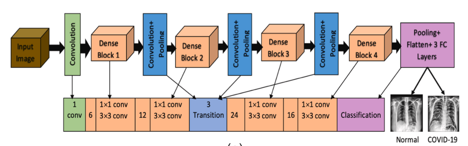图：分类任务更强调整图诊断模式；检测则进一步把可疑区域显式定位出来。

---

核心方法

这一节只抓住 4 个关键点。

1. 先判断任务到底要全图标签还是候选位置

如果目标是筛查、分流、初步告警，分类通常就够用；如果后续需要医生快速复核病灶位置，检测会更合适。

2. 把高召回放在前面

医学任务里，特别是筛查场景，往往宁可多报一些可疑样本，也不能轻易漏掉严重病灶。

3. 认真处理类别不平衡

阳性样本少是常态。重采样、加权损失、阈值调整，往往比单纯换 backbone 更先影响结果。

4. 让输出可解释、可复核

概率、热力图、混淆矩阵、ROC/AUC、错例分析，都是医生判断模型是否可靠的重要依据。

---

典型案例

场景 1：胸部 X 光二分类或多标签分类

• 目标：正常/异常、肺炎、积液、结节等标签预测。
• 难点：阳性比例低，而且很多异常区域很小。
• 本地源码：src/ch05/medical_image_classification/main.py。

场景 2：病灶检测作为分诊入口

• 目标：给出候选病灶框，供医生或后续分割模型复核。
• 适合：肺结节、乳腺钙化、骨折可疑点等。
• 本节重点：先建立分类直觉，再理解检测为何需要额外学习位置。

场景 3：模型解释与错误分析

• 目标：不仅看总体分数，还要知道模型到底看到了哪里。
• 建议输出：预测概率、混淆矩阵、ROC/AUC、热力图或注意力图。
• 本地结果文件：src/ch05/medical_image_classification/output/medical_classification_report.json。

---

实践提示

正文只保留帮助理解的关键片段；完整网络、训练循环和结果可视化请看本地脚本。

1. 最小分类头

import torch.nn as nn


def classification_head(in_features, num_classes):
    return nn.Sequential(
        nn.Linear(in_features, 256),
        nn.ReLU(inplace=True),
        nn.Dropout(0.5),
        nn.Linear(256, num_classes),
    )

2. 类别不平衡时的加权交叉熵

import torch
import torch.nn.functional as F


def weighted_ce(logits, targets, class_weights):
    return F.cross_entropy(logits, targets, weight=torch.tensor(class_weights))

3. 从 logits 到可读概率

import torch


def to_probabilities(logits):
    return torch.softmax(logits, dim=1)

4. 做分类/检测时优先补上的检查

• 不要只看 accuracy，同时看 recall、precision、F1、AUC；
• 单独分析假阳性和假阴性；
• 检查热力图是否真的落在病灶附近；
• 明确分类模型和检测模型在临床流程中的分工。

---

小结

这一节学会了：分类和检测的作用，是在不追求精细轮廓时，先完成筛查、分流和粗定位。

理解了这一节之后，你会更容易判断：某个任务到底应该先做分类、直接做检测，还是需要再走到分割那一步。

代码实验 / 实践附录

运行命令、环境依赖、完整输出和可运行 demo 已统一迁移到 5.6 代码实验 / 实践附录 与 src/ch05/README.md。