Chapter 7: The Truth About Complexity: It's Not About Speed, It's About Structure

P≠NP (if it holds) tells us not that "some problems are hard," but that "the universe itself has a certain asymmetry."

I. An Asymmetry

In 2023, while DeepSeek-R1 and GPT-4 were breaking records on various reasoning tasks, researchers began testing their performance on NP-complete problems. The results were shocking.

[Zixi Li, 2025a] designed the OpenXOR test—a diagnostic tool based on constraint satisfaction. The task is simple: given a set of XOR-style constraint satisfaction instances, determine whether there exists an assignment that satisfies all constraints. Note that this is not the pure XOR-SAT from linear algebra that can be solved by Gaussian elimination, but rather an OpenXOR diagnostic task designed with a combinatorial search structure: it preserves the local deceptiveness of "XOR relations" while pushing the solving into the phase transition region of NP-hard search.

NP-Complete Problems: Why Are They So Much Harder Than Ordinary Hard Problems? (Pallas's Cat Original Research: OpenXOR, Zixi Li 2025)

NP (Nondeterministic Polynomial): A class of problems—given a candidate answer, you can verify whether it is correct in polynomial time. For example, 3-SAT: given a variable assignment, you can quickly check whether it satisfies all clauses.

P (Polynomial): Another class of problems—you can directly find the answer in polynomial time. For example, sorting, shortest path (Dijkstra).

NP-complete: The hardest batch of problems in NP—so hard that if you can efficiently solve any one of them, you can efficiently solve all NP problems.

P = NP? This is the most famous open problem in computer science. Most believe P ≠ NP—that is, verification is far easier than search, and these two capabilities are fundamentally different. But no one can prove it.

Why can't LLMs solve NP-complete problems? Because LLM reasoning is polynomial-time (limited forward propagation steps), while NP-complete problems require exponential search—the problem collapses as scale grows. This is a fundamental architectural limitation, not a parameter count issue.

The test results were astonishing. DeepSeek-R1's task completion rate was 0%. GPT-4's task completion rate was also 0%. Meanwhile, a symbolic solver called OpenLM with only 100k parameters achieved an accuracy of 76%.

Note that this is not 0% accuracy, but a 0% task completion rate—the models either refused to answer (37-42%), hit context limits (28-31%), or hallucinated constraints (18-22%). They didn't even attempt to solve the problem.

This result reveals a profound fact: scale is not the key issue; architecture is.

But why? How can a hundred-billion-parameter model fail at a problem that a 100k-parameter symbolic solver handles correctly?

There is a crucial fact here: an LLM's forward propagation is polynomial-time—no matter how large the model, the amount of computation in a single forward pass is bounded by the product of the number of layers $L$ and sequence length $N$ , at $O (L N^{2})$ . And the OpenXOR test instances were not chosen randomly: their constraint density was carefully controlled around $α \approx 4.26$ —a phase transition critical point that we will discuss in detail shortly. At this point, 3-SAT instances abruptly shift from "almost always satisfiable" to "almost always unsatisfiable," and solvers are trapped precisely in the hardest search region.

The symbolic solver OpenLM used backtracking and propagation—essentially performing exponential search, efficiently organized by 100k parameters. LLMs have no search, only forward propagation. A polynomial-time architecture, confronting an exponential-difficulty problem, yields a 0% task completion rate. Scale can help you do more complex pattern matching in polynomial time, but it cannot turn polynomial time into exponential time. This is an architectural boundary, not a computational power boundary.

Let us begin understanding this asymmetry from the most fundamental level.

II. Verification and Search: A Simple Experiment

Take out a piece of paper and write down this 3-SAT instance:

(x₁ ∨ ¬x₂ ∨ x₃) ∧ (¬x₁ ∨ x₂ ∨ ¬x₄) ∧ (x₂ ∨ x₃ ∨ x₄) ∧ (¬x₁ ∨ ¬x₃ ∨ x₄)

Now I'll give you a candidate solution: x₁=True, x₂=False, x₃=True, x₄=True.

Verify whether it satisfies all clauses:

First clause: x₁=True, satisfied.

Second clause: ¬x₁=False, x₂=False, ¬x₄=False... wait, this clause is not satisfied.

So this is not a solution. How long did the entire verification process take you? 10 seconds? 20 seconds?

Now, without looking at the answer, find an assignment that satisfies all clauses from scratch.

You might try:

x₁=True, x₂=True, x₃=True, x₄=True check not satisfied
x₁=True, x₂=True, x₃=True, x₄=False check not satisfied
x₁=True, x₂=True, x₃=False, x₄=True check not satisfied
…

With 4 variables, there are 2⁴=16 possibilities. If you're unlucky, you may need to try all 16 to find a solution (or confirm there is none).

This is the asymmetry between verification and search. Verifying a candidate solution takes O(m) time, where m is the number of clauses—linear time. But searching for a solution takes O(2ⁿ × m) time, where n is the number of variables—exponential time.

When n=10, the search space is 1024. When n=100, the search space is 2¹⁰⁰ $\approx$ 10³⁰—more than the number of atoms in the universe.

This is not an engineering problem; this is a mathematical fact.

III. Do It Yourself: Experience the Exponential Wall

Let's do a more intuitive experiment.

Step 1: Construct a small-scale 3-SAT instance

Variables: x₁, x₂, x₃, x₄ (4 Boolean variables)

Clauses:

(x₁ ∨ ¬x₂ ∨ x₃)
(¬x₁ ∨ x₂ ∨ ¬x₄)
(x₂ ∨ x₃ ∨ x₄)
(¬x₁ ∨ ¬x₃ ∨ x₄)

Step 2: Verify a candidate solution

Given assignment: x₁=T, x₂=F, x₃=T, x₄=T

Check clause by clause (each clause needs at least one literal to be true):

Clause 1: x₁=T, satisfied
Clause 2: x₂=F, satisfied
Clause 3: x₂=F, x₃=T, satisfied
Clause 4: ¬x₁=F, ¬x₃=F, x₄=T, satisfied

Verification passed! Time: O(4) = constant time.

Step 3: Search all possible solutions

Now, without looking at the answer, enumerate all 2⁴=16 assignments:

python

from itertools import product

# Define 4-variable 3-SAT instance
# Each clause is a list of literals; positive i means x_i, negative -i means ¬x_i
clauses = [
    [1, -2, 3],   # (x₁ ∨ ¬x₂ ∨ x₃)
    [-1, 2, -4],  # (¬x₁ ∨ x₂ ∨ ¬x₄)
    [2, 3, 4],    # (x₂ ∨ x₃ ∨ x₄)
    [-1, -3, 4],  # (¬x₁ ∨ ¬x₃ ∨ x₄)
]

def check_clause(clause, assignment):
    """Check if a single clause is satisfied: at least one literal is true"""
    for lit in clause:
        # lit > 0 means positive literal, lit < 0 means negated literal
        val = assignment[abs(lit) - 1]
        if (lit > 0 and val) or (lit < 0 and not val):
            return True
    return False

def check_sat(clauses, assignment):
    """Check if all clauses are simultaneously satisfied"""
    return all(check_clause(c, assignment) for c in clauses)

# Enumerate all 2^4 = 16 assignments (False=0, True=1)
print(f"{'x₁':^5}{'x₂':^5}{'x₃':^5}{'x₄':^5}{'Satisfied?':^8}")
print("-" * 35)
solutions = []
for bits in product([False, True], repeat=4):
    sat = check_sat(clauses, bits)
    mark = "Yes" if sat else "No"
    vals = ["T" if b else "F" for b in bits]
    print(f"{vals[0]:^5}{vals[1]:^5}{vals[2]:^5}{vals[3]:^5}{mark:^8}")
    if sat:
        solutions.append(bits)

print(f"\nFound {len(solutions)} satisfying assignments:")
for sol in solutions:
    print("  ", {f"x{i+1}": ("T" if v else "F") for i, v in enumerate(sol)})

Experience exponential growth:

5 variables → 32 assignments
10 variables → 1,024 assignments
20 variables → 1,048,576 assignments

Step 4: Thought exercise

If the number of variables increases to 100, how long would exhaustive enumeration take?

Assuming 10⁹ assignments checked per second (modern CPU speed), it would require:

\frac{2^{100}}{10^{9}} \approx 4 \times 10^{13} seconds \approx 1.27 million years

The age of the universe is 13.8 billion years. You would need one ten-thousandth of the age of the universe to solve a 100-variable 3-SAT instance.

This is the exponential wall.

IV. Phase Transition: Where Problems Are Hardest

But not all 3-SAT instances are equally hard.

This sounds like stating the obvious. Of course they're not equally hard—a 10-variable instance is simpler than a 100-variable instance. But that's not what I'm talking about.

What I mean is: even when the number of variables is the same, different 3-SAT instances can differ dramatically in difficulty. And this difference is not random—it follows a pattern.

Consider two extremes. The first extreme is the under-constrained case: 10 variables, 20 clauses, clause density $α = 2$ . There are few constraints, and the solution space is large. Throw a random assignment in, and you'll likely hit a solution. The solver barely needs to backtrack.

The second extreme is the over-constrained case: 10 variables, 80 clauses, clause density $α = 8$ . There are too many constraints, and contradictions surface quickly. The solver discovers after a few steps that "this path won't work," prunes quickly, and switches paths. Although there is no solution, proving unsatisfiability is fast.

Neither extreme is hard.

But around $α \approx 4.26$ , something strange happens.

[Xu & Li, 2000], in their groundbreaking work in 2000, discovered: when the clause density $α = m / n$ increases from 2 to 8, the probability of satisfiability does not decline smoothly.

At $α \approx 4.26$ , a sharp phase transition occurs.

From near 1, it plunges to near 0. Not a gradual decay, but a cliff-like drop.

This is not the first time we've seen phase transitions in computational problems. But every time we see it, it is unsettling. Because it means that the nature of the problem undergoes a qualitative change at a certain critical point. Just as water changes from solid to liquid at 0°C, just as a magnet loses its magnetism at the Curie temperature, 3-SAT at $α \approx 4.26$ shifts from "almost always satisfiable" to "almost always unsatisfiable."

More importantly, this phase transition point is precisely where problems are hardest to solve.

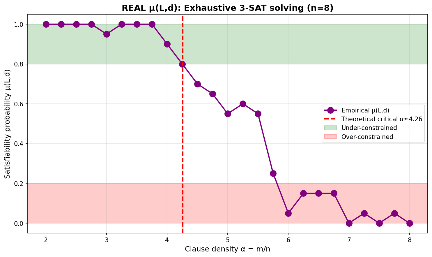Figure 7.2: 3-SAT Phase Transition Diagram Horizontal axis: clause density $α = m / n$ , vertical axis: probability of satisfiability for random instances. The S-shaped curve undergoes a sharp phase transition at $α \approx 4.26$ . The green shaded region ( $α < 4.2$ ) is the under-constrained zone, almost always satisfiable. The red shaded region ( $α > 4.3$ ) is the over-constrained zone, almost always unsatisfiable. Near the critical point (yellow region) is the hardest region to solve.

Why is the critical point the hardest?

Let me first explain the two extreme cases.

In the under-constrained zone, the number of solutions is large. Random search easily hits one. The solver doesn't need to be very clever, just needs not to be too unlucky.

In the over-constrained zone, contradictions surface quickly. The solver discovers after a few steps that "this path won't work," backtracks, prunes, and switches paths. Although it ultimately proves there is no solution, the process is fast.

But at the critical point, the solver falls into a delicate balance.

The number of solutions is small, but not zero. So you can't give up the search. Contradictions are not obvious enough, so the backtracking tree becomes enormous. The search space is neither sparse nor dense—it is precisely in the state hardest to navigate: you can find neither shortcuts nor quickly eliminate wrong directions.

This is the worst kind of predicament.

[Zhan, 2026] explained this phenomenon using a discrete geometric model. He mapped 3-SAT to the combinatorial topology of the N-dimensional Boolean hypercube, deriving the minimum unsatisfiability limit as $α = 8 / N$ , and the maximum satisfiability limit as $α = 7 / 6 (N - 1) (N - 2)$ .

This explains why the satisfiability threshold conjecture only holds "almost surely"—at finite scales, the phase transition is not absolute but probabilistic.

V. μ(L,d): Making Discrete Boundaries Continuous

The problem with traditional complexity theory is that it only tells us whether a problem "belongs to" P or NP, but cannot quantify how hard a specific instance is.

3-SAT is NP-complete—a binary verdict. But this does not mean all 3-SAT instances are equally hard. An instance with 10 variables and 20 clauses is vastly different in difficulty from one with 100 variables and 420 clauses.

[Zixi Li, 2025a]'s OpenXOR framework breaks through this limitation. It transforms the solvability of NP problems from a binary verdict into a continuous phase diagram.

For an instance of scale L and constraint density d, define the solvability probability μ(L,d):

μ (L, d) = \frac{1}{2} (1 - erf (\frac{d - d_{c} (L)}{0.1007}))

where the critical constraint density satisfies the logarithmic scaling law:

d_{c} (L) = - 0.0809 \ln (L) + 0.501

The beauty of this formula lies in three points. First, universality: all phase transition curves across different scales collapse into a single kernel function. Second, predictability: given L and d, one can predict the solvability probability without actual solving. Third, continuity: $μ \in [0, 1]$ , not a binary verdict of "solvable" or "unsolvable."

Experimental validation: on 22,000 OpenXOR instances, this formula achieves a mean squared error MSE~10⁻³.

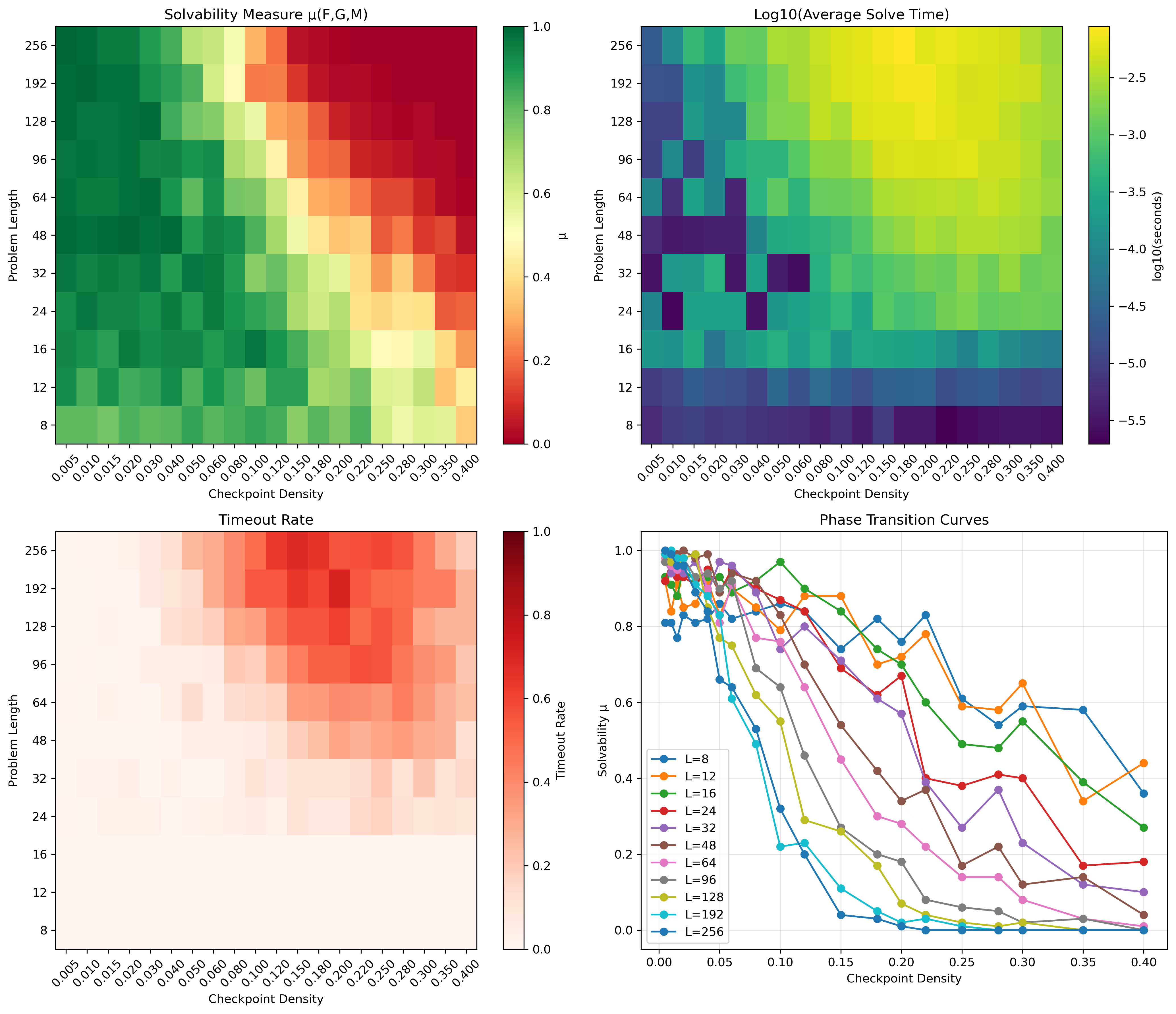
Figure 7.3: μ(L,d) Continuous Phase Diagram

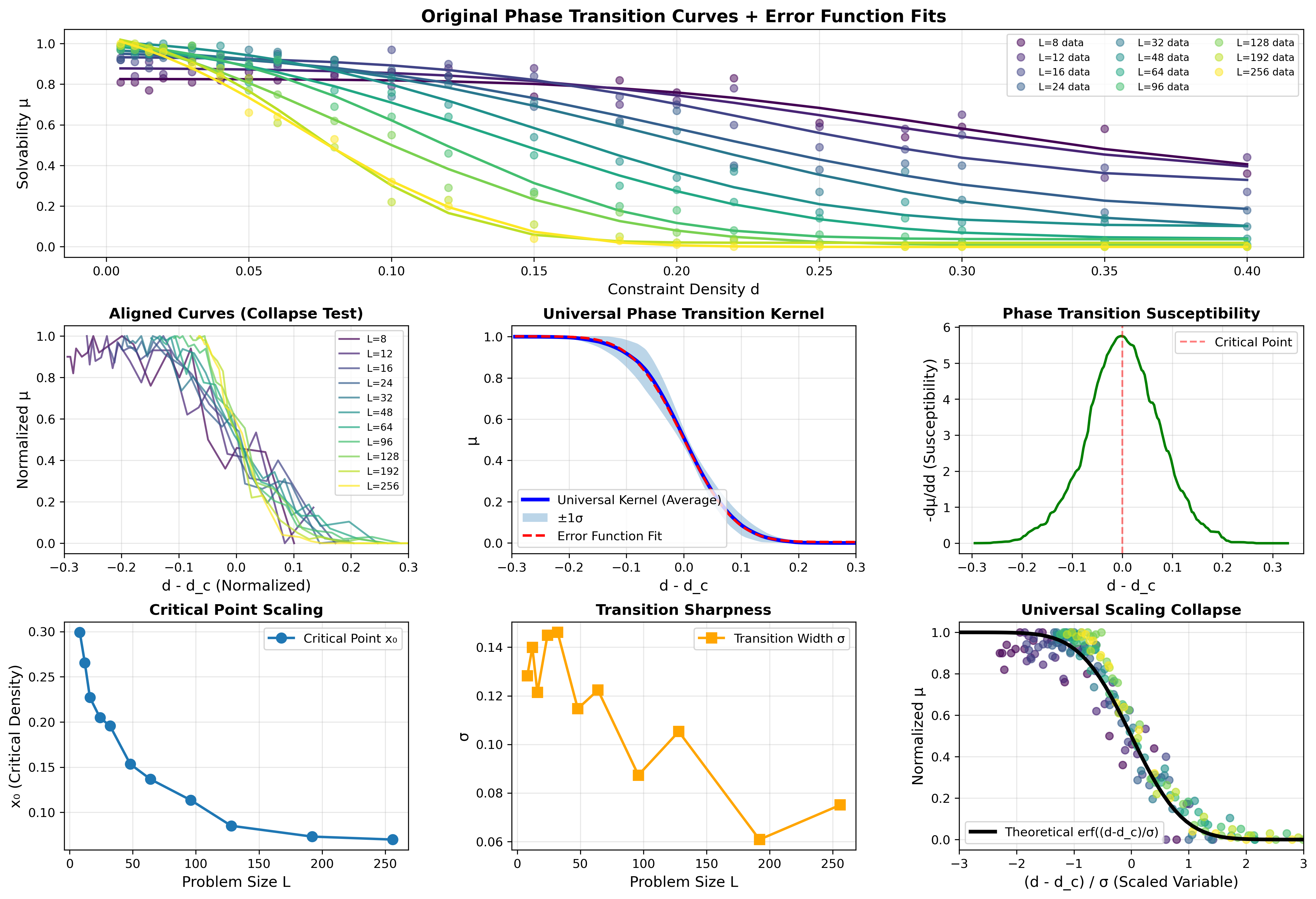
OpenXOR phase diagram: horizontal axis is constraint density d, vertical axis is problem scale L. Color represents solvability probability $μ (L, d)$ , from deep blue ( $μ \approx 0$ , nearly unsolvable) to deep red ( $μ \approx 1$ , almost always solvable). The white curve is the critical boundary $d_{c} (L)$ , along which $μ \approx 0.5$ . The phase transition kernel function transforms the discrete P/NP boundary into a continuous probability landscape.

Figure 7.4: Universal Kernel Function

All phase transition curves across different scales collapse into a single error function kernel. This universality indicates that the "shape" of the phase transition is scale-independent; only the critical point position shifts with ln(L).

This reveals a philosophical shift: computability is not binary, but probabilistic.

Traditional complexity theory is like a political map: this problem belongs to P, that problem belongs to NP, with clearly drawn boundaries. But the real distribution of instances is more like a weather map. You cannot only ask "which country does this belong to"; you must also ask "what is the visibility here, in which direction is the storm moving, is the temperature crossing a critical point?"

What $μ (L, d)$ does is to turn the political map into a weather map. It does not overthrow the P/NP classification, but supplements it with what the reader truly needs: how close a specific instance is to the edge of collapse.

Why is $μ (L, d)$ more informative than "this is NP-complete"? "3-SAT is NP-complete" only tells you that in the worst case there is no known efficient algorithm. It does not tell you whether a specific instance will be quickly solved by a solver.

$L$ denotes scale, $d$ denotes constraint density, $d_{c} (L)$ denotes the critical density at this scale. Then:

When $d ≪ d_{c} (L)$ : too few constraints, many solutions, even random search easily hits the answer;
When $d ≫ d_{c} (L)$ : too many constraints, contradictions surface quickly, pruning is highly effective;
When $d \approx d_{c} (L)$ : solutions are sparse but not absent, contradictions exist but are not obvious, the search tree is maximal.

So the hardest instances are not the "largest" ones, but the ones "closest to the phase transition." This is precisely the significance of OpenXOR: it does not intimidate models with scale, but places them on the thinnest, most dangerous ice of the complexity landscape.

NP is not a wall but a gradient fog. At the edge of the fog ( $μ \approx 0.5$ ), problems exist in a quantum superposition of solvable and unsolvable. Tiny parameter changes can lead to qualitative leaps.

VI. NP-Completeness: The Cook-Levin Theorem and Reduction

P vs NP is an existence question—we don't know the answer. But with this question unresolved, mathematicians did something clever: prove that certain problems are "as hard as all NP problems."

This is NP-completeness.

6.1 The Cook-Levin Theorem: SAT is NP-Complete

In 1971, Stephen Cook (and independently, Leonid Levin) proved a stunning theorem:

SAT (the Boolean satisfiability problem) is NP-complete.

SAT asks: given a Boolean formula (a logical expression composed of AND/OR/NOT), does there exist a variable assignment that makes it true?

For example: $(x_{1} \lor \neg x_{2}) \land (\neg x_{1} \lor x_{3}) \land (\neg x_{2} \lor \neg x_{3})$

Does there exist an assignment to $x_{1}, x_{2}, x_{3}$ that makes the entire formula true?

The Cook-Levin theorem says two things:

First, SAT belongs to NP: given an assignment, verifying whether it satisfies the formula takes only $O (n)$ time. Verification is easy; search (finding the assignment) may be hard.

Second, all NP problems can be reduced to SAT: for any NP problem $X$ , any instance of $X$ can be transformed in polynomial time into a SAT instance, such that: the original instance has a solution $⟺$ the SAT instance is satisfiable.

The direction of reduction is key: it's not that SAT is as hard as $X$ , but that SAT is at least as hard as $X$ —because you can use a SAT solver to solve $X$ .

If someone invents a polynomial-time algorithm for SAT, they simultaneously solve all NP problems.

In 1971, Cook did something smarter than proving P≠NP. He didn't know whether P and NP are equal—to this day no one knows. But he proved that SAT is the ceiling of all NP problems. If you can break through the SAT ceiling, the entire NP edifice collapses into P.

This is the power of reduction: you don't need to defeat each NP problem one by one—3-SAT, Traveling Salesman, Knapsack, Graph Coloring… each is different, each is hard. But reduction tells you that they all share the same "hardness structure." Defeat one, defeat them all.

6.2 Polynomial Reduction: The Transmission of Hardness

The core tool of NP-completeness is polynomial-time reduction.

Problem $A$ reduces in polynomial time to problem $B$ (denoted $A \leq_{p} B$ ), meaning:

There exists a polynomial-time algorithm $f$ such that $x \in A ⟺ f (x) \in B$ .

Intuition: if you can solve $B$ , you can use $f$ to transform instances of $A$ into instances of $B$ , then solve them using $B$ 's algorithm, and translate the answer back. The cost is only the polynomial transformation time.

Reduction chain: Cook proved SAT is NP-complete. Then, Richard Karp (1972) gave reduction chains for 21 classic problems:

SAT \leq_{p} 3-SAT \leq_{p} Independent Set \leq_{p} Vertex Cover \leq_{p} Set Cover \leq_{p} \dots

Each reduction step proves the new problem is NP-complete.

This reduction chain has a philosophical meaning: these seemingly unrelated problems are equivalent in computational hardness. Graph theory, combinatorial optimization, logical reasoning… at their base they share the same "hardness structure."

6.3 Why This Matters for Reasoning

NP-completeness tells us:

If P≠NP, then there does not exist a universal efficient reasoning algorithm.

Theorem proving, planning problems, constraint satisfaction… most of these reasoning tasks are NP-complete. This means:

Exact algorithms are exponential in the worst case
Heuristics (Chapter 8) and approximation algorithms (also Chapter 8) are the only practically viable paths
No algorithm can simultaneously achieve: generality, efficiency, and exactness

Of these three, you can only choose two. This is not an engineering limitation; it is a mathematical theorem.

VII. The Halting Problem: The Ultimate Forbidden Zone of Computation

If P vs NP is a question about "hardness," then the halting problem is a question about "possibility."

These two boundaries are fundamentally different. P vs NP asks: how much harder is search than verification? Even if P≠NP, you can still brute-force search—it just takes exponential time; it draws a line in the time dimension. The halting problem asks: will this program halt? Even given infinite time and infinite memory, no algorithm can answer—it seals off the answer in the logical dimension.

One measures with time, one seals with logic. The two boundaries of computation do not overlap.

It is not that certain problems are very hard to solve; it is that certain problems cannot be solved at all.

The halting problem asks: given a program P and its input x, can one determine whether P(x) will halt (rather than loop forever)?

In 1936, Turing proved this problem undecidable using a diagonalization argument. Let us reproduce this proof.

Assume: there exists a halting decider H(P, x) that can determine whether program P halts on input x.

Construct: define a new program D:

Contradiction: now ask, will D(D) halt?

If H(D, D) returns "halts," then D(D) will enter an infinite loop, not halting
If H(D, D) returns "does not halt," then D(D) will return immediately, halting

In either case, H's judgment is wrong. Therefore H cannot exist.

The profundity of this proof lies not in its technique, but in the structural limitation it reveals.

The halting problem is undecidable not because:

We haven't found a clever enough algorithm yet
Computers aren't fast enough yet
We need more memory

But because no algorithm can solve it. This is logical necessity, not technical limitation.

[Hamkins & Nenu, 2024] conducted a detailed historical analysis of Turing's original paper. They point out that while Turing's 1936 paper indeed contained the core ideas of undecidability, the modern formulation of the halting problem was gradually refined later. This reminds us that even the most foundational theoretical results have a historical evolution more complex than we imagine.

The halting problem demarcates the ultimate boundary of computation. Beyond this boundary, it is not "hard"—it is "impossible."

VIII. The Philosophical Meaning of Complexity

What complexity theory tells us is not just "which problems are hard," but rather the computational structure of the universe.

P vs NP asks: is the asymmetry between verification and search fundamental? If P≠NP holds, it means there exists a fundamental asymmetry in the universe—knowing the answer is easier than finding it, and this gap cannot be bridged by any algorithm.

This is not a technical question, but a question about the nature of knowledge. Why is verification easier than discovery? Why is understanding easier than creation? What does this asymmetry suggest?

The phase transition kernel function μ(L,d) tells us that this asymmetry is not absolute, but asymptotic. Near the phase transition point, problems exist in a critical state between solvable and unsolvable. Tiny parameter changes can lead to qualitative leaps—from "almost always solvable" to "almost always unsolvable."

The halting problem demarcates the ultimate boundary of computation. Some problems are not "hard" but "impossible." This is not a technical limitation, but logical necessity. Any sufficiently powerful computational system will encounter this boundary.

Some problems are too hard to solve exactly. In the next chapter, we will see how heuristic algorithms bypass this wall using "approximations with explicit cost"—and what contracts those approximations must honor.

Open Questions

Can P≠NP be proved? Or is it itself an undecidable proposition? If P≠NP is unprovable, what would that mean?
Can the phase transition kernel function be generalized? Can the μ(L,d) framework be extended to other complexity classes, such as PSPACE, EXP? Do phase transitions across different problems follow a unified mathematical structure?
Computational phase transitions in nature — Protein folding, neural network training, biological evolution: do these natural computational processes also follow similar phase transition laws?
The architectural flaw of LLMs — Why can a 100k-parameter symbolic solver achieve 76% accuracy, while a hundred-billion-parameter LLM achieves a 0% task completion rate? Where exactly is the gap?

Chapter 7: The Truth About Complexity: It's Not About Speed, It's About Structure ​

I. An Asymmetry ​

II. Verification and Search: A Simple Experiment ​

III. Do It Yourself: Experience the Exponential Wall ​

IV. Phase Transition: Where Problems Are Hardest ​

V. μ(L,d): Making Discrete Boundaries Continuous ​

VI. NP-Completeness: The Cook-Levin Theorem and Reduction ​

6.1 The Cook-Levin Theorem: SAT is NP-Complete ​

6.2 Polynomial Reduction: The Transmission of Hardness ​

6.3 Why This Matters for Reasoning ​

VII. The Halting Problem: The Ultimate Forbidden Zone of Computation ​

VIII. The Philosophical Meaning of Complexity ​

Open Questions ​

Further Reading ​