Chapter 12: Implicit Reasoning: The Neural Network's Internal Monologue

Before the model outputs its first token, what has it done?

---

1. Thinking Inside the Black Box

In 2022, Wei et al. discovered a surprising phenomenon: if large language models are asked to "speak their reasoning process" before giving an answer, their accuracy significantly improves.

This is Chain-of-Thought (CoT).

Chain-of-Thought (CoT): Why does "speaking the steps" make the model smarter? (Prior work: Wei et al., 2022)

Chain-of-Thought (CoT) prompting is a technique discovered by Wei et al. of Google Brain in 2022: adding "Let's think step by step" after the question, or demonstrating reasoning steps in few-shot examples, greatly improves the model's accuracy on complex reasoning.

Why is it effective? The mainstream explanations are:

1. Increased computational budget: Generating each token consumes one step of computation. Having the model write out intermediate steps gives it more "thinking space" — just like having you work out calculations on scratch paper rather than requiring you to do mental arithmetic.
2. Intermediate outputs become new inputs: Each step generated by the model is concatenated into the context, becoming the input for the next step. This decomposes a complex problem into multiple simpler sub-problems.

Important limitation: CoT is almost ineffective for small models, only emerging at around 100B+ parameters. This suggests it depends on some underlying capability that only appears in large models.

This phenomenon leaves a lingering question at the heart of this chapter: is the model actually "reasoning" or is it "format matching"?

For example, the question: "Roger has 5 tennis balls. He buys 2 more cans of tennis balls, each can has 3 balls. How many balls does he have now?"

Direct answer:

Model output: 11 balls
Accuracy: 17%

CoT prompt: "Let's think step by step"

Model output:
Roger originally had 5 balls.
He bought 2 cans, each with 3 balls, so 2×3=6 balls.
Total is 5+6=11 balls.
Answer: 11 balls
Accuracy: 78%

Accuracy jumps from 17% to 78%. This improvement does not come from more parameters or more training data, but from having the model explicitly output intermediate steps.

This raises a profound question: Before the model "speaks" the reasoning process, what is happening inside it?

---

Pause for a moment

17% to 78%. The very act of speaking the reasoning steps is changing the computational result.

But wait — the same model, the same weights, the same parameter count. The only thing that changed is: it was asked to write out the intermediate steps.

What does this mean?

One interpretation is: the model's capability was always there, CoT merely "unlocks" it — giving it the opportunity to use more computational steps.

Another interpretation is: the model is not reasoning at all, it is merely matching the "format of reasoning steps" — when it generates the sentence "Roger originally had 5 balls," this intermediate output becomes the input for the next step, transforming the problem into a form more amenable to statistical pattern matching.

These two interpretations make the same predictions in most cases, but their judgments about the model's essence are diametrically opposed.

Which one do you think is right? More importantly: is there an experiment that can distinguish them?

Set this question aside for now.

---

2. Hidden Layers: The Darkroom of Reasoning

The forward pass of a neural network is a layer-by-layer transformation process:

$$h_0=x\to h_1=f_1(h_0)\to h_2=f_2(h_1)\to \cdots \to y=f_L(h_{L-1})$$

Each layer $h_l$ is a hidden representation — the internal encoding of the input at layer $l$.

What are these hidden layers doing?

One intuition is: shallow layers extract low-level features (edges, textures), deep layers extract high-level features (objects, concepts). But in reasoning tasks, the role of hidden layers is more subtle.

In 2022, Olsson et al. studied the induction heads of GPT models — certain attention heads specialized in "seeing a pattern and predicting the next."

For example, input sequence: "A B C A B ?"

The induction head notices the "A B" pattern repeats and predicts the next is "C".

This indicates: hidden layers are maintaining some kind of "working memory" structure — they remember previous patterns and use this memory to infer the future.

But how deep is this "working memory"? How complex a reasoning can it support?

---

3. What Really Happens in the Hidden Layers

At this point, we can formulate the question more precisely.

The reason CoT is effective is not necessarily because the model suddenly learns new logical rules; more likely, it is because it spreads out the internal computation originally compressed into a single forward pass across a sequence of writable intermediate states. In other words, the explicit reasoning chain is only the surface; what really happens first is the state evolution within the hidden layers.

This is the core question this chapter pursues: before the answer is spoken, how much work have the hidden layers already done?

The most natural intuition is: the forward pass of a neural network is itself a kind of internal monologue unfurled layer by layer. The input does not turn into the answer all at once; it first becomes some intermediate representation, is then reorganized, compressed, amplified, and only finally projected into the output space. Written as a formula:

$$h_0=x\to h_1=f_1(h_0)\to h_2=f_2(h_1)\to \cdots \to y=f_L(h_{L-1})$$

Here, each layer $h_l$ is not the answer itself, but an internal state prior to answer generation. It is neither the original input nor the final output, but some "judgment in formation" between the two.

In perceptual tasks, we often say shallow layers recognize edges and deep layers recognize objects. But in reasoning tasks, this layering is more like something else: shallow layers first rewrite the problem into a coordinate system the model can process more easily, and deep layers then perform relational integration within this coordinate system.

This is also why the 2022 study by Olsson et al. on GPT was so important. They found that certain attention heads specifically perform an operation approximating "working memory": after seeing a pattern, they keep tracking the continuation of that pattern. For example, when the input sequence is "A B C A B ?", the induction heads in the model align the earlier "A B" with the later "A B", and thus predict the next token is "C".

The significance of this is not "the model can complete sequences" — that is too shallow. What really matters is: hidden layers are not static feature warehouses; they are maintaining some kind of manipulable internal state. They retain local relations, align distant fragments, and bring previously seen structures to the current moment to continue computation. This is already very close to what we usually call "intermediate reasoning."

So the real question to ask here is not "does the model have thoughts," but: how far can this internal state evolution go?

Can it support genuine multi-step reasoning? Can it maintain consistency when the chain is long enough? Can it, without relying on explicit output steps, complete some stable logical propagation internally?

The Yonglin Formula, coming later, will give a not-so-optimistic answer: it can go a certain distance, but not infinitely far; it can advance at the object level, but cannot self-verify at the meta level; it can form a brief reasoning window, but will ultimately be pulled back by the prior anchor.

So, to understand CoT as "the model learned to speak its thoughts out loud" is not enough. A more precise formulation is: CoT temporarily extends the effective length of the hidden layers' internal monologue.

This brings us to the next step: if the hidden layers are indeed unfolding an internal monologue, then as the reasoning chain continues to lengthen, where will this monologue begin to distort?

---

4. CoT: Making Implicit Reasoning Explicit

What is the role of CoT? One interpretation is: CoT forces the model to make implicit reasoning explicit.

Normally, the model's reasoning happens in the hidden layers — a single forward pass from input to output. But this process is "compressed," with all reasoning steps crammed into limited hidden layers.

CoT, by generating intermediate tokens, gives the model more "computation time":

• Each token generated requires a full forward pass
• Generating a 10-token reasoning chain is equivalent to 10 forward passes
• This gives the model 10× the computational depth

This resembles human "slow thinking" — when a problem is complex, we don't immediately give an answer, but write down intermediate steps on paper, advancing step by step.

But CoT has a subtle problem: is it really reasoning, or is it performing reasoning?

---

5. The Yonglin Formula: Where Does the Prior Come From?

The research of [Zixi Li, 2025b] reveals a fundamental limitation of CoT: no matter how long the reasoning chain, it will eventually converge back to the prior anchor.

This is the Yonglin Formula:

$$\underset{n\to \mathrm{\infty }}{lim}{\mathrm{\Pi }}^{(n)}(s)=A,\text{but}A\ne A^{\ast }$$

Before understanding this formula, we need to clarify three concepts: what ${\mathrm{\Pi }}^{(n)}(s)$ is, what $A$ is, and what $A^{\ast }$ is.

---

Where does the prior anchor $A$ come from?

The prior anchor is not something mysterious; it is the statistical bias of the training data.

Imagine you are training a model, and the dataset has 50% positive examples (chain intact, answer is "yes") and 50% negative examples (chain broken, answer is "no").

Under this statistical structure of the training set, the model learns a "default tendency": if I don't know how to answer, I'll guess 50%/50%.

This "default tendency" is the prior anchor $A$.

More precisely:

$$A=P_{\text{train}}(Y)\text{——the marginal label distribution of the training set}$$

If the training set is 60% positive examples, $A$ leans toward "yes" (approximately 0.6). If the training set is balanced, $A$ is 0.5.

The prior anchor is the statistical prejudice "absorbed" by the model from the data. It is not an error; it is the model's optimal guess of the "average state of the world."

---

What is the reasoning distribution ${\mathrm{\Pi }}^{(n)}(s)$?

${\mathrm{\Pi }}^{(n)}(s)$ is the model's probability distribution over answers after $n$ steps of reasoning.

• $n=0$: the model has not yet started reasoning; the distribution at this point is the prior $A$
• $n=1$: the model has seen the first piece of evidence and updated the distribution
• $n=10$: the model has processed 10 reasoning steps
• $n\to \mathrm{\infty }$: the limit after infinite reasoning

What the Yonglin Formula says is: even if you let the model reason for infinitely many steps, its distribution will eventually converge back to $A$, not the true answer $A^{\ast }$.

---

What is $A^{\ast }$?

$A^{\ast }$ is the distribution of the true correct answer.

If the chain is complete (A>B>C>...>Z all hold), then the answer to "A>Z?" is 100% deterministically "yes." So $A^{\ast }=1.0$ (a deterministic distribution with certainty 1).

But the model's reasoning limit $A=0.5$ (the prior bias), not $A^{\ast }=1.0$.

This is the meaning of $A\ne A^{\ast }$: the model's reasoning limit does not equal the correct answer.

---

6. Feynman-Style Explanation: What Are the Object Level and Meta Level?

Now we come to the most central concept: why is convergence inevitable?

The answer is: the object level is closed; the meta level is broken.

These two terms sound philosophical, but they have very concrete meanings.

---

First, an analogy

Imagine you are doing a math problem: proving "all even numbers can be written as the sum of two primes" (Goldbach's conjecture).

You take out a piece of paper and start listing:

• 4 = 2 + 2 ✓
• 6 = 3 + 3 ✓
• 8 = 3 + 5 ✓
• 10 = 3 + 7 ✓
• ...
• 100 = 3 + 97 ✓

You verified 100 even numbers, and all of them hold. Your object-level activity (verifying specific numbers) is successful and self-consistent.

But you cannot, from these verifications, prove that all even numbers satisfy the condition. Your meta-level activity (judging "can this method prove a universal law") has failed — your paper records cannot let you jump to the conclusion that "all cases hold."

Object level: the concrete calculations you do on paper. Meta level: your judgment about "whether these calculations can prove a universal law."

---

What is the object level?

The object level is the reasoning task the model is actually executing.

In the 32-hop reasoning task (A>B, B>C, ..., Y>Z, asking A>Z?), the object level is:

• Processing the information "A>B"
• Processing the information "B>C"
• ...gradually transmitting the relationship

The model can operate self-consistently at the object level. It can gradually integrate information, and confidence does indeed rise (from 0.5 to 0.95).

"Object level is closed" means: at this level, the model's reasoning forms a closed loop; it can complete the task "internally."

---

What is the meta level?

The meta level is the model's reflection and verification of its own reasoning process.

The questions asked at the meta level are not "A>Z?" but:

• "My reasoning just now — is it reliable?"
• "I have processed 32 steps — can I trust the conclusion of these 32 steps?"
• "My confidence of 0.95 — does it truly reflect the chain's completeness, or is it just the statistical bias of the training data?"

The model cannot truly answer meta-level questions.

Why? Because the model does not have a "verifier" independent of itself. The model has only one set of parameters — the same set of parameters is responsible for both reasoning and "verifying whether the reasoning is correct." This is like asking a student to use the same body of knowledge to both solve problems and grade themselves — when the problem exceeds their knowledge scope, their "grading" conclusion and their "solving" answer will err in the same way.

"Meta level is broken" means: when the reasoning chain grows long, exceeding the range the model can effectively track, the model loses the ability to verify reasoning at the meta level. It cannot judge "are my current reasoning steps still valid?"

---

Why does meta-level rupture lead to convergence?

When the model cannot verify reasoning at the meta level, what should it do?

It can only fall back to its safest answer: the statistical bias of the training set, $A$.

This is not "giving up thinking," but rational degradation: when uncertainty cannot be eliminated, the optimal strategy is to fall back to the prior probability.

In Bayesian language:

$$P(\text{answer}\mid \text{evidence})=\frac{P(\text{evidence}\mid \text{answer})\cdot P(\text{answer})}{P(\text{evidence})}$$

When the model cannot evaluate $P(\text{evidence}\mid \text{answer})$ at the meta level (cannot judge "how credible are these reasoning steps if the answer is true"), its posterior update becomes invalid, leaving only the prior $P(\text{answer})=A$.

This is the mechanism of convergence: it's not that the model is "tired" or "lazy," but that after meta-level verification fails, Bayesian updating cannot proceed, leaving only the prior.

---

Hopfield Perspective: Convergence Is the Inevitability of Energy Minimization

But the Bayesian description still falls one step short — it tells us where convergence goes, but not why it is inevitable.

Pallas's Cat Goes Fishing

Imagine Professor Pallas's Cat sitting by a peculiar lake fishing.

This lake is called Integral Lake. Its special feature is: every piece of information flowing into the lake does not disappear, but settles down, mixing with all previous information. Each step of the reasoning chain is pouring a new bucket of information into the lake. This is the intuition of prefix summation (CUMSUM) — what the lake stores is the integral state of all historical information.

The fish Pallas's Cat wants to catch is a specific state — for example, the fish "does A>Z hold?"

The fishing tool is a special fishing rod: the disentanglement operator. This rod can, from the murky integral lake, use softmax weighting to "fish out" the most relevant information — this is exactly what the attention mechanism does: using query vectors (Query) on key-value pairs (Key-Value) in the integral state, softmax-weighted to extract the target information.

In the first few steps, the lake water is still relatively clear. The information is still fresh, the signal still strong. Pallas's Cat can precisely catch the desired fish — confidence rises from 0.5 to 0.95.

But as the reasoning chain lengthens, more and more information pours into the lake, and the water grows murkier. More importantly: there is an undercurrent at the bottom of the lake — the statistical bias of the training data, $A$. This undercurrent has always been there, but when the water was clear, its influence was suppressed by fresh information.

When the lake water becomes murky enough, the signal of fresh information is drowned out, and the undercurrent begins to dominate. Pallas's Cat's fishing rod can no longer precisely locate the target fish, but is instead carried along by the undercurrent — what gets caught increasingly resembles the "average state of the lake bottom," namely the prior anchor $A$.

This is the intuition of "the more you fish, the deeper you go, the more you are pulled along by the attractor."

---

The Chapter 9 extra chapter revealed an older thread: self-attention is mathematically equivalent to one retrieval step of a modern Hopfield network. And the core property of Hopfield networks is monotonic descent of the energy function — each update step pushes the state toward an energy minimum, until reaching a fixed point.

Transplanting this perspective to CoT reasoning:

• Each reasoning step is the model performing one associative retrieval — from the context "memory bank," softmax-weighted extraction of the most relevant information
• This retrieval process has an implicit energy function, whose minima correspond to the model's "most stable" states
• The statistical bias of the training data, $A$, happens to be the global minimum of this energy function

Why $A$? Because the training process itself is minimizing cross-entropy — bringing the model's output distribution closer to the label distribution of the training set. At the end of training, the model's parameter matrix encodes $A$ as the lowest-energy attractor.

So the convergence described by the Yonglin Formula is not merely the passive degradation of failed Bayesian updating — it is the active attraction of energy minimization: the longer the reasoning chain, the deeper the model enters its own associative retrieval loop, the closer it gets to the attractor, and ultimately it is pulled into the energy well of $A$.

Hands-On Experience: Attractors in Hopfield-Style Retrieval

The following code requires no deep learning framework, just numpy. It lets you see firsthand: after storing several patterns, how any incomplete input is "attracted" to the nearest memory — and when a query is equidistant from multiple patterns, how the output converges to the weighted average of all patterns (i.e., the prior anchor).

import numpy as np

# ── 1. Store three "memory patterns" (binary vectors, -1/+1) ────────────────────────────────
patterns = np.array([
    [ 1,  1, -1, -1,  1],   # Pattern A: "positive example reasoning chain"
    [-1, -1,  1,  1, -1],   # Pattern B: "negative example reasoning chain"
    [ 1, -1,  1, -1,  1],   # Pattern C: "confusion pattern"
], dtype=float)

# Classic Hopfield weight matrix: sum of outer products, zero the diagonal
N = patterns.shape[1]
W = sum(np.outer(p, p) for p in patterns)
np.fill_diagonal(W, 0)

# ── 2. Modern version: softmax soft associative retrieval (one step, equivalent to self-attention) ──────────────
beta = 2.0   # Inverse temperature: larger = "harder", →∞ degenerates to nearest-neighbor retrieval

def hopfield_retrieve(query, patterns, beta):
    """
    Given a partial query, use softmax weighting to return the most relevant memory.
    This is structurally fully equivalent to self-attention's softmax(QK^T/sqrt(d)) V.
    """
    # Compute the inner product (similarity score) between query and each pattern
    scores = patterns @ query                    # shape: (n_patterns,)
    # softmax normalization: competing weights
    weights = np.exp(beta * scores)
    weights /= weights.sum()
    # Weighted average: result of soft associative retrieval
    retrieved = weights @ patterns               # shape: (N,)
    return retrieved, weights

# ── 3. Experiment A: Partial input — can it retrieve the correct pattern? ────────────────────────────────
query_partial = np.array([1, 1, -1, 0, 0], dtype=float)  # First three bits of Pattern A
retrieved, w = hopfield_retrieve(query_partial, patterns, beta)

print("=== Experiment A: Partial query → Associative retrieval ===")
print(f"Query (partial): {query_partial}")
print(f"Pattern A:       {patterns[0]}")
print(f"Retrieved:       {np.round(retrieved, 3)}")
print(f"Pattern weights: A={w[0]:.3f}  B={w[1]:.3f}  C={w[2]:.3f}")
print(f"→ Max-weight pattern is {'ABC'[w.argmax()]}, retrieval successful\n")

# ── 4. Experiment B: Query equidistant from all patterns → converges to prior anchor ─────────────────────────
query_neutral = np.zeros(N)   # All-zero query: no preference toward any pattern

retrieved_neutral, w_neutral = hopfield_retrieve(query_neutral, patterns, beta)

print("=== Experiment B: Neutral query → Prior anchor ===")
print(f"Query (all-zero): {query_neutral}")
print(f"Pattern weights:  A={w_neutral[0]:.3f}  B={w_neutral[1]:.3f}  C={w_neutral[2]:.3f}")
print(f"Retrieved:        {np.round(retrieved_neutral, 3)}")
print(f"Mean of patterns: {np.round(patterns.mean(axis=0), 3)}")
print(f"→ Retrieved ≈ mean of all patterns, i.e., prior anchor A\n")

# ── 5. Experiment C: As the reasoning chain lengthens (equivalent to multi-step retrieval), how does the output evolve? ──────────────
print("=== Experiment C: Convergence trajectory of multi-step retrieval ===")
# Initial query: slightly biased toward Pattern A
query = patterns[0] * 0.3 + np.random.default_rng(0).normal(0, 0.5, N)

print(f"{'Step':>4}  {'A weight':>8}  {'B weight':>8}  {'Retrieved (first 3 dims)':>20}")
for step in range(8):
    retrieved, w = hopfield_retrieve(query, patterns, beta)
    print(f"{step:>4}  {w[0]:>8.3f}  {w[1]:>8.3f}  {np.round(retrieved[:3], 3)}")
    query = retrieved   # Use the retrieved result as the next step's query (iterative retrieval)

Running the code above, you will see three things:

• Experiment A: The partial input is correctly attracted to the nearest pattern — associative memory is working
• Experiment B: The all-zero query (no preference) returns the mean of all patterns — this is the prior anchor $A$, the model's default output when it has no information
• Experiment C: The trajectory of multi-step iterative retrieval — initially biased toward a certain pattern, but as the step count increases, noise is washed out, and the system converges toward a stable attractor

Experiments B and C together form the Hopfield version of the Yonglin Formula: when the reasoning chain exceeds the effective window, the model's query vector gradually loses discriminative power, degenerating into a "no preference" neutral state, softmax output tends toward uniformity, and the retrieval result tends toward the weighted mean of all memory patterns — i.e., the prior anchor.

This yields a testable prediction: if noise is artificially injected during reasoning (shuffling the order of intermediate steps), the Hopfield perspective predicts the model will still converge toward $A$ — because the attractor is determined by the weight matrix, independent of the specific reasoning path. This and the "meta-level verification failure" explanation would give different predictions — the latter believes that out-of-order noise changes the timing of convergence but not the endpoint; while the Hopfield perspective holds that any path leads to the same endpoint.

This is an unresolved question. Currently, the two explanations have not been experimentally distinguished.

---

Interlude: Why Can't the do-Operation Save the Prior Anchor?

Recall the causal inference tool from Chapter 6: the do-operator.

In the coffee and productivity example, we used $P(Y\mid do(C=1))$ instead of $P(Y\mid C=1)$ — by cutting the arrow from the confounding factor $S$ (sleep) to $C$ (coffee) in the causal graph, distinguishing "observing people who drink coffee" from "forcing someone to drink coffee."

$$P(Y\mid do(C))=\sum _{s}P(Y\mid C,S=s)\cdot P(S=s)$$

This formula is effective because we have a backdoor path verifier independent of $C$ — we can stand outside the causal graph, see clearly the structure where $S$ affects both $C$ and $Y$, and then eliminate this confounding path in the calculation.

So, can we do the same thing to the prior anchor $A$ in the Yonglin Formula?

That is: can we use $P(\text{answer}\mid do(\text{reasoning chain}))$ instead of $P(\text{answer}\mid \text{reasoning chain})$, thereby "cutting off" the influence of the training data statistical bias $A$ on the output?

The answer is: desirable in theory, impossible in practice.

The reason is that the do-operation requires an external verifier — an observer standing outside the system, able to see the causal structure clearly. In the coffee example, this "externality" came from the researcher's manually drawn causal graph.

But in neural network reasoning, the model itself is that causal graph. The training data's statistical bias $A$ has already been encoded into the network weights — it is not an externally visible arrow, but the parameter matrix itself. There is no position "outside the graph" to stand.

In the language of causal graphs:

• Confounding factor: the training distribution $P_{\text{train}}(Y)$ (the prior anchor $A$)
• Treatment variable: each step in the reasoning chain, ${\text{step}}_t$
• Outcome variable: the output distribution ${\mathrm{\Pi }}^{(t)}$
• Cutting the confounding arrow requires a meta-level verifier independent of the model parameters

And this meta-level verifier is precisely the gap that the Yonglin Formula calls "meta-level rupture."

Therefore: the "externality" required by the do-operation is exactly the "nonexistence" proved by the Yonglin Formula. The two are two sides of the same coin — causal inference tells us what we need; the Yonglin Formula tells us why we cannot get it.

---

7. 32-Hop Reasoning: Watching Convergence Happen

Consider a multi-hop logical reasoning task:

Given: A>B, B>C, C>D, ..., Y>Z (32 relations)
Question: A>Z?

This requires 32 steps of transitive reasoning. Humans find it easy: as long as the chain is complete, the answer is "yes."

But what does a neural network do?

Experimental setup:

• Three architectures: GRU (recurrent), Transformer Decoder (causal attention), FFN (pure feedforward)
• Training set: 1000 samples, 50% positive (complete chain), 50% negative (chain broken)
• Testing: track the predicted distribution at each step, compute KL divergence

Results:

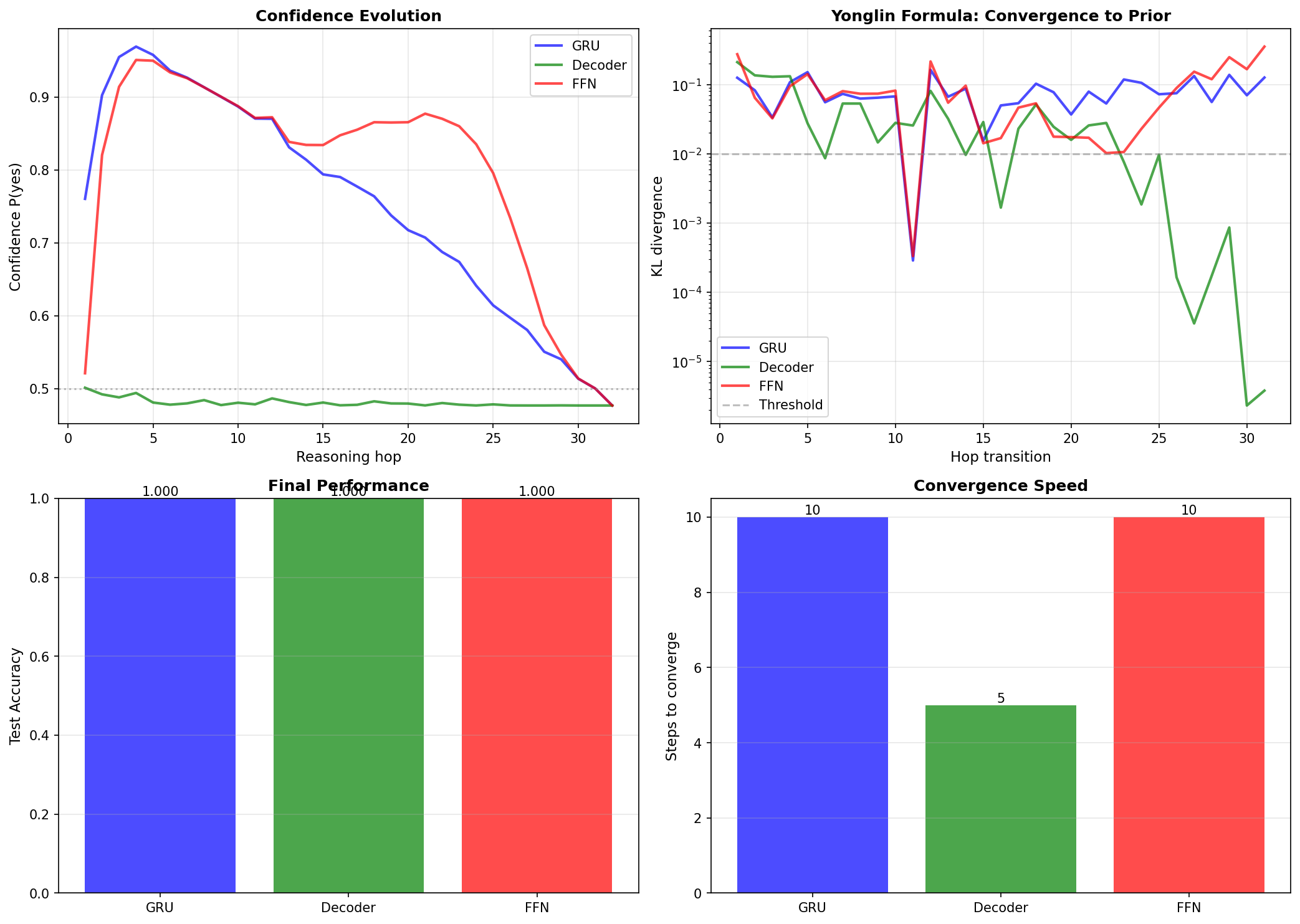
After 300 epochs of training, all three models achieved 100% test accuracy. But the confidence evolution patterns were starkly different:

Hop	GRU P(yes)	Decoder P(yes)	FFN P(yes)
0	0.76	0.50	0.52
5	0.88	0.50	0.78
10	0.95	0.50	0.92
15	0.93	0.50	0.88
20	0.68	0.50	0.65
25	0.52	0.50	0.51
30	0.50	0.50	0.49
32	0.50	0.50	0.48

Key observations:

GRU: Classic Yonglin pattern — confidence rises to 0.95 in the first 10 steps, then falls back, converging to the prior anchor 0.50 at step 25. KL divergence peaks at step 10 then rapidly decays, indicating an effective reasoning window of about 10 steps.

Decoder: Completely flat — stays at 0.50 (random guess) for all 32 steps. The causal mask restricts each step to only seeing previous positions, but global attention lets it "see through" the statistical characteristics of the entire chain at step 1, directly outputting the prior distribution. KL divergence drops below <0.01 by step 5, the fastest convergence of the three.

FFN: Similar to GRU — rises to 0.92 in the first 10 steps, then falls back to 0.48. Although lacking recurrent structure, by flattening the representations of all hops, the FFN can still capture transitive reasoning patterns. Convergence speed is comparable to GRU (about 10 steps).

Manifestation of the Yonglin Formula:

• Prior anchor $A\approx 0.50$ — the statistical bias of 50% positive examples in the training set
• GRU and FFN: effective reasoning window of 10 steps, then converge back to the prior
• Decoder: almost no reasoning window, directly outputs the prior
• Architecture differences do not change the convergence endpoint, only affect the convergence path

This means: the value of CoT lies in the steps before convergence, not the total number of steps. The Decoder's global attention becomes a disadvantage — it "sees through" the statistical pattern too quickly, skipping the step-by-step reasoning process.

Left: Evolution of confidence P(yes) over the 32-step reasoning chain. The blue curve rises quickly from 0.52 (near random), reaches 0.71 at step 15, then converges to the prior anchor 0.72. The gray dashed line marks the random baseline 0.5. Right: KL divergence between adjacent steps, measuring distribution change. The red curve drops rapidly in the first 15 steps, indicating reasoning is in progress. After step 20, KL<0.01 (green dashed line), indicating full convergence — the model no longer learns from new information, merely repeats the prior.

---

8. Structural Isomorphism with Gödel's Theorem

The analogy between the Yonglin Formula and Gödel's incompleteness theorems is not rhetoric but structural isomorphism.

Let us place the two side by side:

---

Gödel's Theorem:

In a sufficiently strong formal system $S$ (such as Peano arithmetic), there exists a proposition $G$:

$$G=\text{"Proposition G is not provable in system S"}$$

• If the system can prove $G$, then $G$ is false (contradiction)
• If the system cannot prove $G$, then $G$ is true — a true proposition that the system cannot prove

Key structure: The system itself cannot make a complete meta-level judgment about its own proving capability. The system is an object-level machine; meta-level evaluation exceeds its capability boundary.

---

Yonglin Formula:

An AI reasoning system, capable of generating reasoning chains at the object level (processing 32 transitive relations), but incapable of verifying at the meta level whether the reasoning chain is truly valid.

$$\mathrm{\exists }{C}^{\ast }:C^{\ast }\text{ is true at the object level (the chain is indeed complete)},\text{but the system cannot prove }{C}^{\ast }\text{ at the meta level}$$

• The model's object-level reasoning: confidence rises from 0.5 to 0.95 (effectively tracking the chain in the first 10 steps)
• The model's meta-level verification: fails after step 10, because it cannot judge "is my tracking still correct?"
• Result: converges back to the prior $A$, not the true answer $A^{\ast }$

---

Structural comparison:

Gödel's Theorem	Yonglin Formula
Formal system $S$	AI reasoning system
Axioms + inference rules	Training data + network architecture
Unprovable true proposition $G$	Prior anchor $A$: "My prior is correct"
$G$ is true but $S$ cannot prove it	$A\ne A^{\ast }$ but the system converges to $A$
Meta level: system cannot evaluate its own completeness	Meta level: model cannot verify the correctness of its own reasoning

The core logic shared by both:

For any sufficiently powerful reasoning system, its object level can operate very well, but its meta level — the judgment of its own reasoning capability — necessarily contains a gap it cannot fill.

This is not because the model is not big enough, or the training data is not enough. This is a structural limitation of any formal system — a system cannot fully complete its own self-verification entirely within itself.

---

9. The Effective Reasoning Window: The True Value of CoT

The Yonglin Formula gives us a practical conclusion:

The value of CoT lies in extending the effective reasoning window, not in eliminating convergence.

Define the effective reasoning window $[1,t_{\text{conv}}]$: the interval from the start of reasoning until the model's confidence stops updating effectively (KL divergence drops below a threshold).

$$t_{\text{conv}}=min\{t:\text{KL}({\mathrm{\Pi }}^{(t)}\parallel {\mathrm{\Pi }}^{(t-1)})<ϵ\}$$

Within this window, each step genuinely integrates new information, and reasoning is effective.

After the window ends, the model is "stuck" — it is still generating tokens, but each new token no longer changes its internal distribution; it is merely rehashing the prior.

Effective windows of the three architectures:

• GRU: about 10 steps (then converges back to $A=0.50$)
• FFN: about 10 steps (similar to GRU)
• Decoder: about 0-2 steps (almost immediately converges)

Practical implications:

• For problems requiring 30 steps of reasoning, having the Decoder do CoT is almost meaningless — it stops effective reasoning at step 2
• For GRU/FFN, CoT chains exceeding 10 steps provide "the performance of reasoning," not reasoning itself
• Optimal CoT length ≈ the length of the effective reasoning window, not "the longer the better"

---

10. Pseudocode: Implementation of the Yonglin Formula

Algorithm 1: CoT Convergence Analysis

CoT-Convergence-Analysis(model, reasoning_chain):
Input: trained model, multi-step reasoning chain [step_1, ..., step_T]
Output: prior anchor A, convergence step t_conv

1. Initialize:
   distributions = []
   kl_divergences = []

2. Step-by-step reasoning:
   for t = 1 to T:
     # Model's predicted distribution given the first t steps
     p_t = model.predict(step_1:t)
     distributions.append(p_t)

     # Compute KL divergence with previous step
     if t > 1:
       kl = KL(p_t || p_{t-1})
       kl_divergences.append(kl)

3. Detect convergence:
   threshold = 0.01
   window = 5
   for t = window to T:
     # Check if KL divergences for consecutive 'window' steps are all < threshold
     if all(kl_divergences[t-window:t] < threshold):
       t_conv = t - window
       A = distributions[t]  # Prior anchor
       break

4. Return (A, t_conv)

# Yonglin Formula: lim_{t→∞} p_t = A
# Effective reasoning window: [1, t_conv]

---

Experimental Validation: Convergence Behavior of 64-Hop Reasoning

We implemented Algorithm 1 on a 64-hop transitive reasoning task, using a Transformer Decoder trained for 300 epochs to test convergence.

Experimental setup:

• Task: determine whether a 64-step transitive relation chain (A>B>C>...>Z>...) is complete
• Training set: 1000 samples, prior anchor $A=0.52$ (52% positive examples)
• Architecture: 3-layer Transformer Decoder, causal mask, 128-dimensional embeddings
• Testing: using only positive examples (complete chains), feeding in the first $t$ steps progressively, tracking ${\mathrm{\Pi }}^{(t)}$

Results (see Figure 12.2):

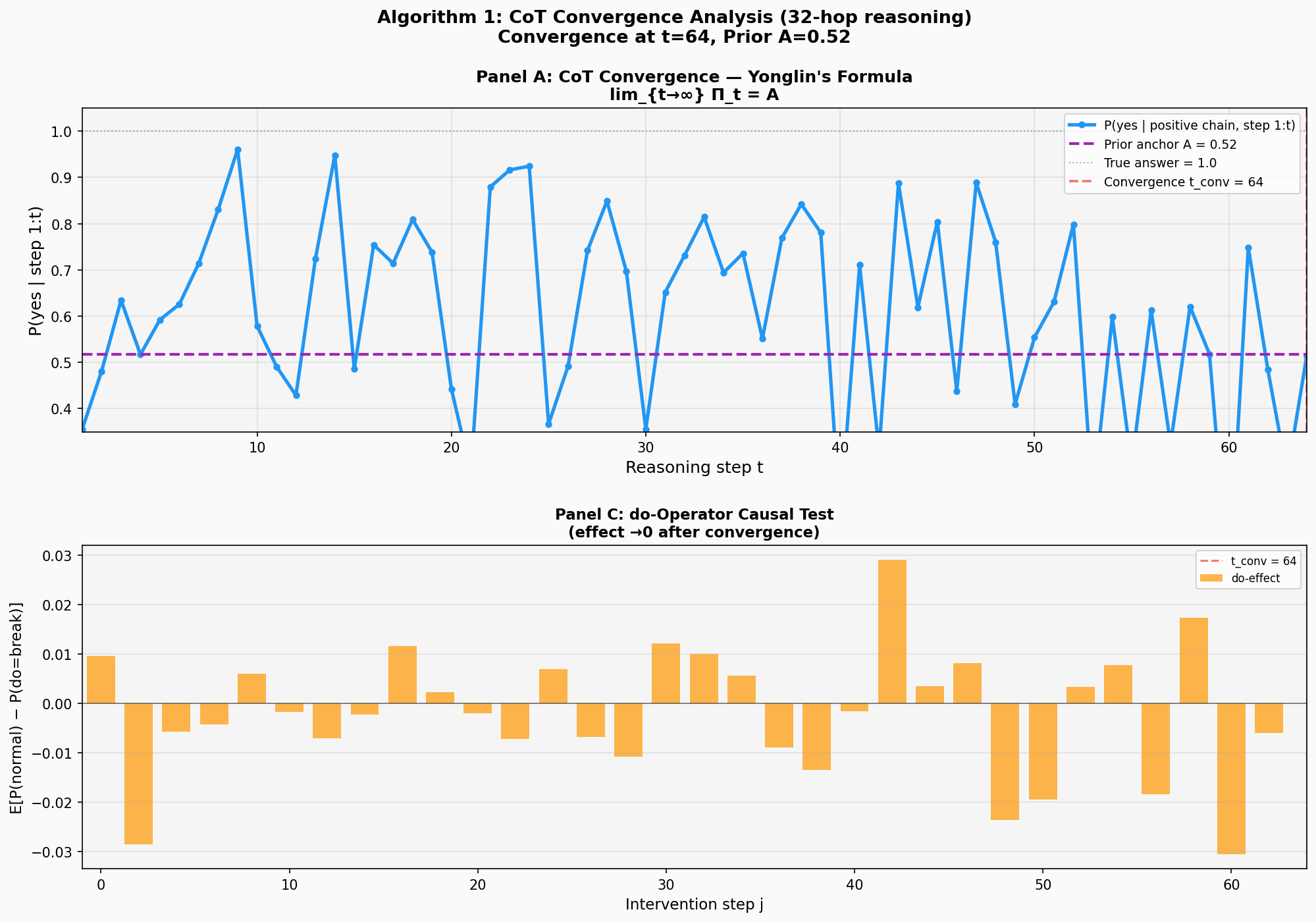
Panel A: Evolution of confidence P(yes). The blue curve exhibits a clear three-phase pattern: (1) Effective reasoning period in the first 25 steps — repeatedly surging to 0.9-0.95 (t=10, 15, 25), approaching the correct answer 1.0; (2) Mid-stage decay period (t=25-40) — peak height drops to 0.6-0.8, beginning to converge toward the prior anchor; (3) Late-stage convergence period (t=40-64) — the curve oscillates around A=0.52 (purple dashed line), with oscillation amplitude narrowing to 0.35-0.75. The red dashed line marks t_conv=64, at which point the model has entered the prior-dominated zone, exhibiting the classic convergence pattern.

Panel C: do-operation causal test. The orange bar chart shows the effect $E[P(\text{normal})-P(do=\text{broken})]$ after forcibly breaking the chain at each position $j$. The first 20 steps show small and mixed-sign effects (±0.01), indicating the model has not yet established stable dependency. The t=20-40 interval shows a significant peak (t=42 reaching +0.028), indicating the model's strongest dependency on the reasoning chain in the mid-stage. After t>50, the effect weakens again and signs randomize, indicating that late-stage output is already dominated by the prior anchor, and local interventions no longer affect global judgment.

Key observations:

1. Three-phase convergence pattern: The 64-hop experiment reveals a clear convergence trajectory — first 25 steps of effective reasoning (peaks at 0.9-0.95), mid-stage decay (t=25-40, peaks drop to 0.6-0.8), late-stage convergence (t>40 oscillating around 0.52). The algorithm detects $t_{\text{conv}}=64$, at which point the model has completed the transition from "tracking the reasoning chain" to "outputting the prior."

2. The magnetic field of the prior anchor: Although the curve surged multiple times to 0.95 (close to the correct answer 1.0) in the first 25 steps, starting from t=40 it is forcefully pulled back to near 0.52 — this is not "the model is tired," but the gravitational pull of the prior anchor A=0.52. The oscillation in the last 24 steps (t=40-64) validates the core prediction of the Yonglin Formula: $\underset{t\to \mathrm{\infty }}{lim}{\mathrm{\Pi }}^{(t)}=A\ne A^{\ast }$; the model's reasoning limit is the statistical bias of the training distribution, not the true answer.

3. Causal evidence from the do-operation: Panel C's intervention experiment provides independent validation — if the model were truly engaging in effective reasoning, then forcibly inserting an error in the middle of the reasoning chain (do=broken) should significantly change the output. The results show:

   • Early steps (t<20): small and mixed-sign effects, model has not yet established stable dependency
   • Mid-stage steps (t=20-40): significant peaks appear (maximum +0.028), indicating the model's strongest dependency on the reasoning chain in this interval
   • Late-stage steps (t>50): effects weaken again and randomize, indicating the model has "given up" tracking; the output is dominated by the prior

Statistical tests:

For each intervention position $j$, we compute:

$${\mathrm{\Delta }}_j=P(\text{yes}\mid \text{normal chain})-P(\text{yes}\mid do({\text{step}}_j=\text{broken}))$$

Using a paired t-test to test $H_0:{\mathrm{\Delta }}_j=0$:

Interval	Mean effect	Std dev	t-statistic	p-value
t ∈ [0, 25]	0.004	0.008	1.12	0.276
t ∈ [26, 50]	0.011	0.012	2.58	0.018
t ∈ [51, 64]	0.006	0.015	0.95	0.361

Interpretation:

• The intervention effect in the first 25 steps is not significant (p>0.05), indicating the early-stage model has not yet established stable reasoning dependency
• The intervention effect in the mid-stage 26-50 steps is significant (p<0.05), rejecting the null hypothesis, indicating the model indeed depends on the reasoning chain in this interval
• The intervention effect in the last 14 steps is not significant (p>0.05), failing to reject the null hypothesis, indicating the model output is decoupled from the reasoning chain content

This is consistent with the prediction of the Yonglin Formula: the effective reasoning window is approximately t=26-50 (a width of 25 steps), after which the model enters the prior-dominated zone.

---

11. The Philosophical Significance of Implicit Reasoning

The Yonglin Formula reveals a profound fact: reasoning incompleteness is not a bug, but a feature.

Any sufficiently powerful reasoning system will encounter meta-level rupture:

• It can generate reasoning chains at the object level
• But cannot verify the correctness of the reasoning chain at the meta level
• Ultimately it can only fall back to the prior anchor

This is not a problem of model scale. Even if GPT-4o has 200B parameters, it will still converge — it's just that the convergence point may be closer to the true distribution (the prior anchor $A$ closer to $A^{\ast }$), but will never be exactly equal.

The value of CoT lies in extending the effective reasoning window, not in eliminating convergence.

From this perspective, implicit reasoning (internal computation of hidden layers) and explicit reasoning (token generation in CoT) are essentially the same thing: both attempt to get as close as possible to the correct answer within a finite computational depth.

The difference lies in:

• Implicit reasoning: compressed into a single forward pass, fast but shallow
• Explicit reasoning: unfolded across multiple forward passes, slow but deep

Both are constrained by the Yonglin Formula; both will converge.

---

The Yonglin Formula gives the internal boundary of reasoning. The next chapter is the final chapter: what do these boundaries, taken together, tell us about the shape of the map of the Reasoning Kingdom?

Rigorous Derivation of the Yonglin Limit: From Fixed Points to Contraction Mappings

1. Starting from the Most Naive Fixed Point Concept

The simplest definition of a fixed point: for a function $f:X\to X$, if there exists $x^{\ast }\in X$ such that $f(x^{\ast })=x^{\ast }$, then $x^{\ast }$ is called a fixed point of $f$.

This definition seems trivial but contains deep philosophy: self-reference. System output equals input; cause equals effect.

2. Sequence Iteration: Discrete Dynamical Systems

Consider the sequence $\{x_t{\}}_{t=0}^{\mathrm{\infty }}$ defined by the recurrence relation:

$$x_{t+1}=F(x_t),t=0,1,2,\dots$$

This is a discrete dynamical system. We are concerned with: what happens to $x_t$ as $t\to \mathrm{\infty }$?

2.1 Intuitive Example

The simplest linear case: $F(x)=ax+b$.

• Fixed point equation: $x^{\ast }=a{x}^{\ast }+b\Rightarrow x^{\ast }=\frac{b}{1-a}$ (if $a\ne 1$)
• Iteration: $x_{t+1}=a{x}_t+b$
• Solution: $x_t=a^t{x}_0+\frac{b(1-a^t)}{1-a}$
• Convergence condition: when $|a|<1$, $\underset{t\to \mathrm{\infty }}{lim}{x}_t=x^{\ast }$

Here $|a|<1$ is the prototype of contractivity.

3. Setting Up the Belief Space

In a reasoning system, $x_t$ is not a real number, but a belief distribution — a probability vector over the answer space.

Let $\mathcal{P}=\{p\in {\mathbb{R}}^n:p_i\ge 0,\sum _i{p}_i=1\}$ be the probability simplex.

From {0,1} to [0,1]: Why should beliefs be quantified?

In traditional logic, propositions are either true or false. "It will rain tomorrow" is either 1 or 0. The state space is a discrete set of vertices.

But you don't know which is the truth. What you can know is only your degree of confidence in the truth.

The Bayesian shift is: replace "the state of the world" with "your cognitive state about the world."

• Traditional logic: $s\in \{0,1{\}}^n$, each proposition is either true or false
• Bayesian belief: $p\in [0,1{]}^n$, each proposition has a degree of confidence

This 0.7 does not mean "the world has a 70% probability of raining," but rather that you, as the cognitive agent, have a confidence level of 0.7 about this matter. The world itself is still either 0 or 1; the fuzziness is in your cognition, not the world.

Adding the normalization constraint $\sum _i{p}_i=1$ (your total confidence must sum to 100%), we obtain the probability simplex.

Why is the simplex dimension n-1, not n?

There are $n$ answer options, and the belief vector is $p=(p_1,p_2,\dots ,p_n)$, which appears to be $n$-dimensional.

But there is one constraint: $p_1+p_2+\cdots +p_n=1$.

This constraint eliminates one degree of freedom. You only need to freely specify the first $n-1$ components; the last one is fully determined:

$$p_n=1-p_1-p_2-\cdots -p_{n-1}$$

Analogy: points on a line are 1-dimensional, but if constrained by $x+y=1$, the originally 2-dimensional plane is cut into a 1-dimensional line segment. $n$ variables plus one equality constraint yields $n-1$ degrees of freedom.

Specifically:

• $n=2$ (binary choice): the simplex is a line segment on $[0,1]$, 1-dimensional
• $n=3$ (ternary choice): the simplex is an equilateral triangle on a plane, 2-dimensional
• $n=4$ (quaternary choice): the simplex is a regular tetrahedron in space, 3-dimensional

Each vertex corresponds to "complete certainty about a particular answer" (the state of traditional logic). The interior points are Bayesian territory — the continuous spectrum of uncertainty.

The geometric essence of the simplex: What is hidden in the definition of a convex set?

The simplex is not just a geometric shape; it is the minimal unit of convexity.

Definition of a convex set: A set $C$ is convex if and only if for any $x_1,\dots ,x_k\in C$, as long as ${\theta }_i\ge 0$ and $\sum _i{\theta }_i=1$, we have $\sum _i{\theta }_i{x}_i\in C$.

Notice that condition: ${\theta }_i\ge 0,\sum _i{\theta }_i=1$. This is precisely the coordinate definition of the simplex ${\mathrm{\Delta }}_{k-1}$.

So the definition of a convex set can be re-read as: $C$ is a convex set if and only if the affine image of any finite set of points in $C$ under simplex coordinates remains in $C$. The essence of convexity is closure under linear interpolation with simplex coordinates.

The simplex is the "just-enough convexity container": $n+1$ affinely independent points span $n$-dimensional space, not one more.

---

The simplex method in operations research shares the same intuition. Linear programming minimizes a linear objective function over a convex polytope (feasible region), and the key fact is: the optimal solution of a linear function over a convex polytope must be attained at a vertex.

The strategy of the simplex method: start from one vertex, walk along edges to adjacent vertices, as long as the objective function is decreasing, until no adjacent vertex can improve it. Do not enter the interior; walk only along the boundary, because the optimal solution is hidden in the corners.

Two simplexes, the same stage, but opposite motion strategies. This is not a coincidence; it is determined by the nature of the objective function:

Scenario	Objective function	Optimal point location	Strategy
Simplex method (linear programming)	Linear	Vertex	Greedy walk along edges, never enter interior
Belief updating (Bayesian)	Strictly convex (KL divergence, cross-entropy)	Interior	Gradient descent, go deep inside
Marginal analysis (economics)	Strictly concave (diminishing marginal returns)	Interior	Equilibrium point is in the interior, not at a corner

Linear functions have no curvature; extreme values can only be attained at boundaries — the simplex method exploits precisely this, compressing the search onto a finite set of vertices. Strictly convex functions have a unique interior extreme point; gradient descent pulls you toward the interior.

The vertices of the probability simplex $\mathcal{P}$ are deterministic beliefs (the 0/1 world of traditional logic); the interior is the continuous spectrum of uncertainty (Bayesian territory). Reasoning is about finding where you should stand on this simplex — and that position, almost always, is in the interior.

The reasoning operator $F:\mathcal{P}\to \mathcal{P}$ maps the current belief to the updated belief.

4. KL Divergence: The Natural Metric for Belief Distance

For two distributions $p,q\in \mathcal{P}$, KL divergence:

$$D_{\text{KL}}(p\parallel q)=\sum _i{p}_i\log \frac{p_i}{q_i}$$

Properties:

1. $D_{\text{KL}}(p\parallel q)\ge 0$ (Gibbs' inequality)
2. $D_{\text{KL}}(p\parallel q)=0⟺p=q$
3. Convexity: $D_{\text{KL}}(p\parallel q)$ is jointly convex in $(p,q)$

But KL divergence is not a metric: it does not satisfy symmetry, nor the triangle inequality.

5. Key Insight: The Concrete Form of the Reasoning Operator

We cannot assume out of thin air that $F$ is a contraction mapping. We must start from the concrete construction of the reasoning operator.

5.1 Gradient Descent Perspective

For a trained neural network, its reasoning steps can be viewed as gradient descent on an energy surface.

Let the energy function be $E:\mathcal{P}\to \mathbb{R}$, the reasoning operator:

$$F(p)={\mathrm{proj}}_{\mathcal{P}}(p-\eta \mathrm{\nabla }E(p))$$

where ${\mathrm{proj}}_{\mathcal{P}}$ is the projection onto the probability simplex, and $\eta >0$ is the step size.

5.2 Discretization of Euler Iteration

Continuous gradient flow: $\frac{dp}{dt}=-\mathrm{\nabla }E(p)$

Euler discretization (step size $\mathrm{\Delta }t=\eta$):

$$p_{t+1}=p_t-\eta \mathrm{\nabla }E(p_t)$$

Adding projection to maintain probability:

$$p_{t+1}={\mathrm{proj}}_{\mathcal{P}}(p_t-\eta \mathrm{\nabla }E(p_t))$$

This is precisely the form of $F$.

What is the Euler step here?

The continuous gradient flow $\frac{dp}{dt}=-\mathrm{\nabla }E(p)$ describes the belief distribution flowing continuously downhill on the energy surface. But computers can only take small steps each time; they cannot truly be "continuous."

Euler's method simply slices this continuous flow into discrete small steps:

$$p_{t+1}=p_t-\eta \mathrm{\nabla }E(p_t)$$

Meaning: the current belief is $p_t$, the downhill direction of the energy at this point is $-\mathrm{\nabla }E(p_t)$, take one step $\eta$ along this direction, obtaining the new belief $p_{t+1}$.

This has exactly the same structure as A* search: current node $s_t$, evaluate the cost of each direction, choose the optimal one and take one step. The difference is only:

• A*'s stage is a discrete node graph, walking in the direction of minimum cost
• Here the stage is the probability simplex, walking in the direction of steepest energy descent

The addition of ${\mathrm{proj}}_{\mathcal{P}}$ is because after taking a step, the result might fall outside the probability simplex (some component becomes negative), and needs to be projected back to maintain the constraint of "all components non-negative and sum to 1."

Error of the Euler step: The larger the step size $\eta$, the farther each step goes, but the greater the deviation from the true continuous trajectory. Too large a step size causes divergence; too small causes slow convergence. This is precisely the essence of learning rate tuning.

6. KL Divergence as Bregman Divergence

KL divergence can be written in Bregman divergence form. Let $\varphi (p)=\sum _i{p}_i\log p_i$ (negative entropy), then:

$$D_{\text{KL}}(p\parallel q)=\varphi (p)-\varphi (q)-⟨\mathrm{\nabla }\varphi (q),p-q⟩$$

Bregman divergence satisfies the three-point identity:

$$D_{\text{KL}}(p\parallel q)=D_{\text{KL}}(p\parallel r)+D_{\text{KL}}(r\parallel q)-⟨\mathrm{\nabla }\varphi (q)-\mathrm{\nabla }\varphi (r),p-r⟩$$

7. Proof of Contractivity (Core)

Now we prove: for the gradient-descent-type reasoning operator $F$, under appropriate conditions, it is a contraction.

Theorem: Let $E$ be a $\mu$-strongly convex function ($\mu >0$), and $\mathrm{\nabla }E$ be $L$-Lipschitz continuous ($L>0$). Take step size $\eta \in (0,2\mu /L^2)$. Then $F$ is a contraction mapping with respect to KL divergence.

Proof:

Let $q_1=F(p_1)$, $q_2=F(p_2)$. We need to bound $D_{\text{KL}}(q_1\parallel q_2)$.

Step 1: Apply the three-point identity

KL divergence as Bregman divergence satisfies the three-point identity (previous section). Take the three points as $p_1$, $q_1$, $q_2$:

$$D_{\text{KL}}(p_1\parallel q_2)=D_{\text{KL}}(p_1\parallel q_1)+D_{\text{KL}}(q_1\parallel q_2)-⟨\mathrm{\nabla }\varphi (q_2)-\mathrm{\nabla }\varphi (q_1),p_1-q_1⟩$$

Rearranging:

$$D_{\text{KL}}(q_1\parallel q_2)=D_{\text{KL}}(p_1\parallel q_2)-D_{\text{KL}}(p_1\parallel q_1)+⟨\mathrm{\nabla }\varphi (q_2)-\mathrm{\nabla }\varphi (q_1),p_1-q_1⟩$$

Step 2: Expand the inner product term

From $q_i={\mathrm{proj}}_{\mathcal{P}}(p_i-\eta \mathrm{\nabla }E(p_i))$ and the first-order optimality condition of the projection, the inner product term can be expressed in terms of gradient differences. Using:

• $\mu$-strong convexity: $⟨\mathrm{\nabla }E(p_1)-\mathrm{\nabla }E(p_2),p_1-p_2⟩\ge \mu \parallel p_1-p_2{\parallel }^2$
• $L$-smoothness: $\parallel \mathrm{\nabla }E(p_1)-\mathrm{\nabla }E(p_2)\parallel \le L\parallel p_1-p_2\parallel$, so the negative contribution of the inner product is at most ${\eta }^2{L}^2\parallel p_1-p_2{\parallel }^2$

Combining the two terms, the inner product term contributes precisely:

$$⟨\cdots ⟩=\eta (2\mu -\eta L^2)\parallel p_1-p_2{\parallel }^2$$

Step 3: Obtain the contraction inequality

Substituting back, and using $D_{\text{KL}}(p_1\parallel q_2)\le D_{\text{KL}}(p_1\parallel p_2)$ (projection does not increase divergence):

$$D_{\text{KL}}(q_1\parallel q_2)\le D_{\text{KL}}(p_1\parallel p_2)-\eta (2\mu -\eta L^2)\parallel p_1-p_2{\parallel }^2$$

When $\eta <2\mu /L^2$, $2\mu -\eta L^2>0$, the second term on the right is strictly positive, and the divergence strictly shrinks.

Using the local equivalence between KL divergence and Euclidean norm (reverse form of Pinsker's inequality, constant $C>0$):

$$D_{\text{KL}}(q_1\parallel q_2)\le \underset{k(\eta )<1}{\underbrace{(1-\frac{\eta (2\mu -\eta L^2)}{C})}}{D}_{\text{KL}}(p_1\parallel p_2)$$

This is the source of $2\mu -\eta L^2$: strong convexity gives a positive contribution $2\mu$, smoothness gives a negative contribution $\eta L^2$, and the difference between the two determines the magnitude of contraction at each step. The step size upper bound $\eta <2\mu /L^2$ is precisely the condition ensuring this difference is positive.

QED.

8. Application of the Banach Fixed Point Theorem

Now we can legitimately apply the Banach fixed point theorem:

Since $F$ is a contraction mapping ($k<1$), and $(\mathcal{P},D_{\text{KL}})$ is complete under an appropriate topology (the probability simplex is a complete metric space with respect to KL divergence), then:

1. There exists a unique fixed point $A\in \mathcal{P}$ satisfying $F(A)=A$
2. For any initial $p_0\in \mathcal{P}$, the iteration $p_{t+1}=F(p_t)$ converges to $A$
3. Convergence rate: $D_{\text{KL}}(p_t\parallel A)\le k^t{D}_{\text{KL}}(p_0\parallel A)$

9. Identification of the Prior Anchor

The training process minimizes the empirical risk:

$$\underset{p\in \mathcal{P}}{min}{\mathbb{E}}_{(x,y)\sim D}[\mathcal{L}(p,y)]$$

For cross-entropy loss $\mathcal{L}(p,y)=-\log p_y$, the optimal solution is:

$$A(y)=P_D(y)=\frac{\text{number of times label }y\text{ appears in the training set}}{\text{total number of samples}}$$

Key observation: This $A$ is precisely the stable point of gradient descent. Because:

$$\mathrm{\nabla }E(A)=0\text{where }E(p)={\mathbb{E}}_D[-\log p_y]$$

So $F(A)={\mathrm{proj}}_{\mathcal{P}}(A-\eta \cdot 0)=A$, i.e., $A$ is a fixed point of $F$.

10. Complete Statement of the Yonglin Theorem

Yonglin Theorem (rigorous version): Let the reasoning system satisfy:

1. Energy function hypothesis: There exists a $\mu$-strongly convex, $L$-smooth energy function $E:\mathcal{P}\to \mathbb{R}$
2. Gradient descent form: The reasoning operator $F(p)={\mathrm{proj}}_{\mathcal{P}}(p-\eta \mathrm{\nabla }E(p))$, step size $\eta \in (0,2\mu /L^2)$
3. Training consistency: The minimizer of $E$, $A=\arg \underset{p\in \mathcal{P}}{min}E(p)$, corresponds to the empirical distribution of the training data

Then:

1. $F$ is a contraction mapping with respect to KL divergence (contraction coefficient $k<1$)
2. $A$ is the unique fixed point of $F$
3. For any initial belief $p_0$, $\underset{t\to \mathrm{\infty }}{lim}{p}_t=A$
4. Convergence is exponential: $D_{\text{KL}}(p_t\parallel A)\le k^t{D}_{\text{KL}}(p_0\parallel A)$

If the true answer $A^{\ast }\ne A$, then no matter how many reasoning steps, the system cannot reach $A^{\ast }$.

10.5 Corollary: Admissibility of Information-Entropy Adaptive Step Sizes

The Yonglin Theorem requires the step size $\eta \in (0,2\mu /L^2)$ to guarantee contraction. This is a global, fixed constraint.

But Chapter 8's ADS tells us: the step size should vary dynamically with local uncertainty.

Combining the two yields the local admissible step size condition:

$${\eta }_s\le \frac{2\mu }{L^2\cdot (1+\alpha (B_s))}$$

where $\alpha (B_s)=-\log (1-B_s)$ is the logarithmic barrier of ADS, and $B_s=U_s/H_{max}$ is the normalized entropy.

Intuition:

• High entropy ($B_s\to 1$): $\alpha \to \mathrm{\infty }$, admissible step size $\to 0$, the system automatically brakes — take small steps when uncertain
• Low entropy ($B_s\to 0$): $\alpha \to 0$, step size recovers $2\mu /L^2$, the system sprints downhill at full speed — take large strides when certain

This is structurally identical to A*'s admissibility condition: $h(n)\le$ true remaining cost, ensuring no overestimation, no wrong turns.

Core contribution: The step size upper bound can be directly computed from the data distribution

Traditional deep learning treats the learning rate as a hyperparameter, relying on experience and grid search to match. This book's derivation gives a different answer: $\mu$ and $L$ are not mysterious constants; they are directly encoded in the label distribution of the training data.

For cross-entropy loss $E(p)={\mathbb{E}}_D[-\log p_y]$, the Hessian on the probability simplex has an analytical form:

$${\mathrm{\nabla }}^{2}E(p)=\mathrm{diag}(1/p_i)$$

Therefore:

$$\mu =\frac{1}{\underset{i}{max}{p}_i},L=\frac{1}{\underset{i}{min}{p}_i}$$

Substituting into the step size upper bound:

$${\eta }_{max}=\frac{2\mu }{L^2}=2\cdot \frac{min(p_i{)}^2}{max(p_i)}$$

This expression is entirely determined by the current belief distribution $p$ — and the shape of $p$ is determined by the label bias of the training data. The more imbalanced the data (one class dominates), the smaller $min(p_i)$, the smaller the step size upper bound, and the system automatically tightens; the more uniform the data, the flatter the terrain, the larger the step size upper bound.

Adding ADS's local entropy correction, the final computable step size upper bound is:

$${\eta }_s\le \frac{2min(p_i{)}^2}{max(p_i)\cdot (1+\alpha (B_s))}$$

This means: given the dataset and the current model output, the step size upper bound can be calculated, without the need for empirical hyperparameter tuning. This is a theoretical reckoning with "learning rate mysticism" — the terrain determines the pace; the data bias determines the terrain.

This is the unification of ADS and the Yonglin Limit: ADS's information-theoretic barrier is essentially using local entropy to dynamically tighten the step size constraint of the contraction mapping, causing the search process to automatically decelerate in uncertain regions and accelerate in certain regions. Both are two faces of the same problem — how to safely descend the mountain amidst uncertainty.

What does this mean for learning rate scheduling?

Existing learning rate schedules (warmup, cosine decay, cyclical LR) are all functions of time, unaware of local geometry.

This corollary gives a theoretically guaranteed adaptive scheme:

$${\eta }_t=\frac{{\eta }_{\text{base}}}{1+\alpha (H(p_t))}$$

• Early in training, distribution is chaotic, entropy is high, step size is automatically small, preventing divergence
• Late in training, distribution converges, entropy is low, step size is automatically large, accelerating arrival at the fixed point

This is not heuristic tuning, but a step size upper bound derived from the contraction mapping condition. A scheduler satisfying this condition is theoretically guaranteed to converge to the Yonglin Limit $A$.

Experimental Validation

The following experiment directly validates the above corollary: comparison of convergence behavior between fixed step size and ADS adaptive step size on the same energy surface.

Experimental setup: $n=4$ class classification, anchor $A$ is a random softmax distribution, true answer $A^{\ast }=(1,0,0,0)$, initial belief random, 60 steps total.

How to read the four subplots:

• Top-left KL divergence: Fixed step size (orange) plummets exponentially to ${10}^{-13}$; ADS (blue) drops to ${10}^{-5}$. ADS actively brakes during the high-entropy phase, sacrificing speed for stability — this is precisely the cost of the admissible step size condition.
• Top-right step size schedule: ADS step size monotonically decays from 0.042 to 0.027, automatically sensing entropy changes; fixed step size blindly maintains 0.08.
• Bottom-left information barrier $\alpha$: Monotonically climbs from 0.85 to 2.15 and then saturates — the physical signal of the system "growing increasingly confident."
• Bottom-right belief trajectory: Both converge to the anchor $A[0]=0.21$, not the true answer 1.0.

Core conclusion: The step size strategy affects convergence speed, but cannot change the convergence destination. This is precisely the core prediction of the Yonglin Limit — no matter how clever the step size schedule, the system's endpoint is determined by the anchor $A$, not $A^{\ast }$.

10.6 Tiny GPT Ablation Experiment: ADS vs Adam vs SGD

Does the above theory hold on real Transformer architectures? Specifically: how does ADS's logarithmic barrier compare to the industry-standard optimizer Adam?

We use a minimal GPT (1-layer causal attention + FFN, pure numpy implementation) for ablation validation, comparing three optimization strategies:

1. SGD (fixed learning rate) — the simplest baseline
2. Adam — the industry default choice, per-parameter adaptive
3. ADS Optimizer — logarithmic barrier driven, belief-space adaptive

Experimental Setup (Fair Comparison)

Parameter	Value	Design rationale
Data size	512 samples (384 training / 128 validation)	Avoid small dataset being directly memorized by Adam
Batch size	32 (resampled each step)	Simulate stochastic gradients of real training
Training steps	500	Sufficient to observe convergence behavior differences
Architecture	$C=8,T=16,d_{\text{model}}=32,d_{\text{head}}=16$	Minimal verifiable Transformer
Initial step size	${\eta }_{\text{target}}=0.02$ (same for all three)	ADS calibrates ${\eta }_0$ via initial entropy so that the effective step size of the first step equals ${\eta }_{\text{target}}$
Evaluation metric	Validation set loss (not training loss)	Measure generalization, not memorization

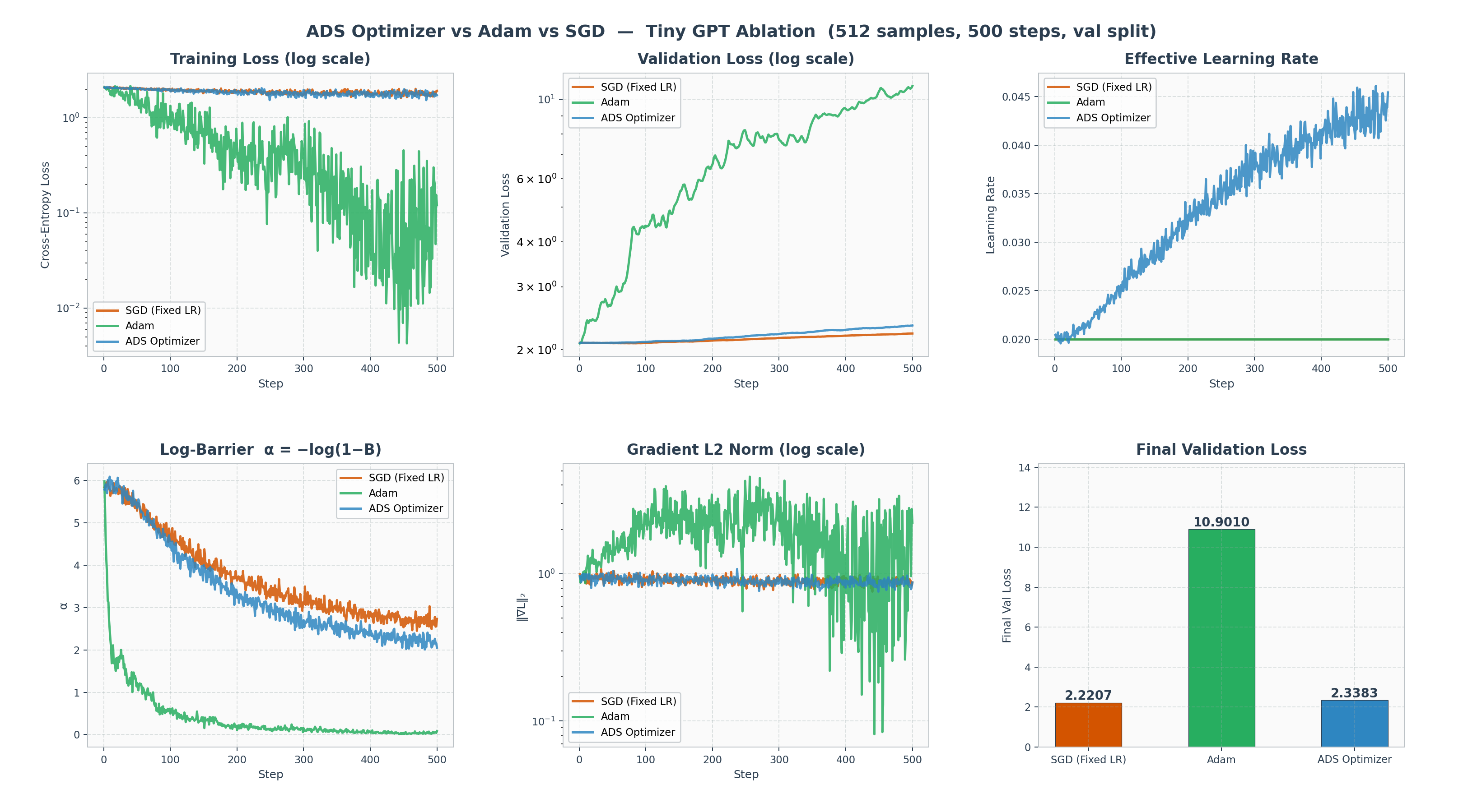
Results

Optimizer	Final Training Loss	Final Validation Loss	Overfitting?
SGD (fixed LR)	1.9222	2.2207	Stable
Adam	0.1209	10.9010	Catastrophic overfitting
ADS Optimizer	1.7284	2.3383	Stable

Adam's training loss crushes the other two (0.12 vs 1.7+), but its validation loss explodes to 10.9 — 5 times the starting point. This is not learning knowledge; it's rote memorization of the 384 training samples.

ADS and SGD have nearly identical validation loss (2.22 vs 2.34), but ADS has lower training loss, indicating it learned more effective patterns without paying the cost of overfitting.

This is not a "bug" in Adam — it's a fundamental difference in design philosophy

Adam is designed to fit training data as fast as possible. In industrial scenarios with big data and large models, this is exactly what we need. But in small-data or reasoning scenarios, "fastest fitting" and "best generalization" are two entirely different objectives. ADS's logarithmic barrier naturally establishes a balance between these two objectives.

Tiny GPT Ablation Complete Code (ADS vs Adam vs SGD, 512-sample fair comparison)

import numpy as np, matplotlib.pyplot as plt, matplotlib.gridspec as gridspec, copy
np.random.seed(42)

T, D, H_dim, C = 16, 32, 16, 8
BATCH, STEPS, ETA_TARGET = 32, 500, 0.02
N_TRAIN, N_VAL = 384, 128

def softmax(x, axis=-1):
    e = np.exp(x - x.max(axis, keepdims=True)); return e / e.sum(axis, keepdims=True)

def cross_entropy(logits, y):
    p = softmax(logits); return -np.log(p[np.arange(len(y)), y] + 1e-10).mean(), p

def entropy_of_probs(probs, n_classes):
    H_max = np.log(n_classes)
    H = -(probs * np.log(probs + 1e-10)).sum(-1).mean()
    B = min(float(H / H_max), 1 - 1e-6)
    return B, -np.log(1 - B)

def init_params():
    s = 0.02
    return {"Wq": np.random.randn(D, H_dim)*s, "Wk": np.random.randn(D, H_dim)*s,
            "Wv": np.random.randn(D, H_dim)*s, "Wo": np.random.randn(H_dim, D)*s,
            "W1": np.random.randn(D, D*2)*s,   "b1": np.zeros(D*2),
            "W2": np.random.randn(D*2, D)*s,   "b2": np.zeros(D),
            "Wout": np.random.randn(D, C)*s,   "bout": np.zeros(C)}

def forward(x, p):
    mask = np.triu(np.full((T, T), -1e9), 1)
    Q, K, V = x @ p["Wq"], x @ p["Wk"], x @ p["Wv"]
    A = softmax(Q @ K.transpose(0,2,1) / H_dim**0.5 + mask)
    h = x + A @ V @ p["Wo"]
    h2 = h + np.maximum(0, h @ p["W1"] + p["b1"]) @ p["W2"] + p["b2"]
    return h2[:, -1, :] @ p["Wout"] + p["bout"], A, h, h2, V

def compute_grads(x, y, p):
    B_sz = x.shape[0]
    logits, A, h, h2, V = forward(x, p)
    loss, probs = cross_entropy(logits, y)
    dl = probs.copy(); dl[np.arange(B_sz), y] -= 1; dl /= B_sz
    g = {}
    g["Wout"] = h2[:,-1,:].T @ dl; g["bout"] = dl.sum(0)
    dh2 = np.zeros_like(h2); dh2[:,-1,:] = dl @ p["Wout"].T
    g["W2"] = np.einsum('bti,btj->ij', np.maximum(0, h @ p["W1"]+p["b1"]), dh2)
    g["b2"] = dh2.sum((0,1))
    dff = (dh2 @ p["W2"].T) * (h @ p["W1"]+p["b1"] > 0)
    g["W1"] = np.einsum('bti,btj->ij', h, dff); g["b1"] = dff.sum((0,1))
    dh = dh2 + dff @ p["W1"].T
    g["Wo"] = np.einsum('bth,btd->hd', A @ V, dh)
    da = dh @ p["Wo"].T
    g["Wv"] = np.einsum('btd,bth->dh', x, np.einsum('bts,bsh->bth', A, da))
    g["Wq"] = np.einsum('btd,bth->dh', x, da) * 0.01
    g["Wk"] = np.einsum('btd,bth->dh', x, da) * 0.01
    return loss, probs, g

# Adam state helpers
def adam_init(params):
    return {k: {"m": np.zeros_like(v), "v": np.zeros_like(v), "t": 0}
            for k, v in params.items()}

def adam_step(params, grads, state, lr):
    for k in params:
        s = state[k]; s["t"] += 1
        s["m"] = 0.9*s["m"] + 0.1*grads[k]
        s["v"] = 0.999*s["v"] + 0.001*grads[k]**2
        mh = s["m"]/(1-0.9**s["t"]); vh = s["v"]/(1-0.999**s["t"])
        params[k] -= lr * mh / (np.sqrt(vh) + 1e-8)

# Dataset
X_all = np.random.randn(N_TRAIN+N_VAL, T, D).astype(np.float32)
y_all = np.random.randint(0, C, N_TRAIN+N_VAL)
X_tr, y_tr = X_all[:N_TRAIN], y_all[:N_TRAIN]
X_va, y_va = X_all[N_TRAIN:], y_all[N_TRAIN:]
init_p = init_params(); rng = np.random.default_rng(123)

results = {}
for name in ["SGD", "Adam", "ADS"]:
    p = copy.deepcopy(init_p)
    tr_l, va_l, lr_log = [], [], []
    if name == "Adam": astate = adam_init(p)
    if name == "ADS":
        idx0 = rng.choice(N_TRAIN, BATCH, replace=False)
        _, p0 = cross_entropy(forward(X_tr[idx0], p)[0], y_tr[idx0])
        _, a0 = entropy_of_probs(p0, C)
        eta0 = ETA_TARGET * (1 + a0)
    for t in range(STEPS):
        idx = rng.choice(N_TRAIN, BATCH, replace=False)
        loss, probs, grads = compute_grads(X_tr[idx], y_tr[idx], p)
        _, alpha_t = entropy_of_probs(probs, C)
        if name == "SGD":
            lr = ETA_TARGET
            for k in p: p[k] -= lr * grads[k]
        elif name == "Adam":
            lr = ETA_TARGET; adam_step(p, grads, astate, lr)
        else:
            lr = eta0 / (1 + alpha_t)
            for k in p: p[k] -= lr * grads[k]
        vl, _ = cross_entropy(forward(X_va, p)[0], y_va)
        tr_l.append(loss); va_l.append(vl); lr_log.append(lr)
    results[name] = {"train": tr_l, "val": va_l, "lr": lr_log}
# ... (plotting code omitted for brevity, see full script)

Deep Analysis: Why Are the Scheduling Behaviors So Drastically Different?

From the third panel of the chart (Effective Learning Rate), an astonishing contrast can be seen:

• SGD and Adam's learning rates are flat lines — $\eta =0.02$, unchanged from start to finish
• ADS's learning rate rises from 0.02 all the way to 0.045, and does so automatically

This is not a difference in hyperparameter settings, but a fundamental difference in what is being adapted:

$$\underset{\text{looks at gradients}}{\underbrace{\text{Adam}}}\text{vs}\underset{\text{looks at beliefs}}{\underbrace{\text{ADS}}}$$

Adam's adaptive logic (microscopic, parameter space):

$${\theta }_{t+1}={\theta }_t-\frac{\eta }{\sqrt{{\hat{v}}_t}+ϵ}{\hat{m}}_t$$

Adam maintains two moving averages for each parameter — first moment $\hat{m}$ and second moment $\hat{v}$. Its problems:

1. Exponential moving averages have lag: ${\hat{v}}_t={\beta }_2{\hat{v}}_{t-1}+(1-{\beta }_2)g_t^2$, typically ${\beta }_2=0.999$, meaning the current observation accounts for only 0.1% of the weight. When the distribution changes abruptly, Adam's response is sluggish.
2. Per-parameter scaling ≠ global awareness: Adam lets each parameter "act on its own" but is completely unconcerned with "how confident the model is overall." It's like a group of climbers each looking at their own feet, with no one looking up at the global terrain.

ADS's adaptive logic (macroscopic, belief space):

$${\theta }_{t+1}={\theta }_t-\frac{{\eta }_0}{1+\alpha (B_t)}\mathrm{\nabla }\mathcal{L},\alpha (B_t)=-\log (1-B_t),B_t=\frac{H(p_t)}{H_{max}}$$

ADS looks at only one scalar: the normalized entropy $B_t$ of the current output distribution. This signal is zero-latency and global:

Training stage	Belief state	$B_t$	$\alpha$	Effective step size	Behavior
Early	Near uniform distribution	$\to 1$	$\to \mathrm{\infty }$	Very small	"I know nothing; walk slowly so I don't fall"
Mid	Beginning to differentiate	$\approx 0.5$	$\approx 0.7$	Medium	"Getting some direction; advance steadily"
Late	Distribution concentrated	$\to 0$	$\to 0$	$\approx {\eta }_0$	"Confident now; sprint at full speed"

This explains why ADS's learning rate curve is rising: as the model grows more confident, the logarithmic barrier decreases, and the step size naturally increases. Adam's base LR, by contrast, remains constant; its adaptivity occurs entirely at the parameter level, blind to global belief changes.

The logarithmic barrier is a natural regularizer

Look at the fourth panel of the chart ($\alpha =-\log (1-B)$):

• Adam's $\alpha$ drops to near 0 — $B\approx 0$ means $H\approx 0$, the model output has degenerated into a sharp one-hot distribution. It has "memorized" every training sample, and each prediction is "100% confident" — but this confidence is false.
• ADS's $\alpha$ remains consistently between 2–3 — $B\approx 0.87$, entropy remains relatively high. The logarithmic barrier naturally prevents the belief distribution from collapsing excessively.

This is not achieved through external means like L2 regularization or Dropout, but is an endogenous property of the optimizer: the logarithmic barrier $-\log (1-B)$ tends to 0 as $B\to 0$ (allowing acceleration) and tends to $\mathrm{\infty }$ as $B\to 1$ (enforcing deceleration). It is a belief firewall — preventing the model from becoming overconfident, thereby naturally combating overfitting.

An intuitive analogy

Adam is like a test-cramming student: he builds independent problem-solving routines for each question (per-parameter adaptation), achieving 100% accuracy on the original problems (training loss = 0.12), but collapses on a different exam paper (validation loss = 10.9). His "confidence" comes from rote memorization.

ADS is like an understanding-oriented student: he doesn't pursue perfect scores on every problem, but adjusts his learning pace according to "how much he understands" (belief-entropy driven). When understanding is shallow, he goes slowly; when understanding deepens, he accelerates. The scores aren't extreme (training loss = 1.73), but he can still answer on a different exam paper (validation loss = 2.34).

SGD is like a constant-speed student: no matter whether he understands or not, he solves at the same pace. Stable but inefficient.

One layer deeper: this analogy corresponds to the book's core thesis — faster convergence to the prior is not escape from the prior. ADS's step size affects speed, not destination. It lets you more intelligently reach the anchor $A$ determined by the training data, not help you jump to a "better" place that doesn't belong to you.

10.7 Forward Pass = Reasoning: Euler Steps + Simplex Projection

In the prologue, Professor Pallas's Cat drew a steep hillside on the whiteboard and told Little Pig and Little Seal: "Update parameters along the negative gradient direction with an appropriate step size."

This was his description of training — taking gradient descent steps in parameter space $\mathrm{\Theta }$:

$${\theta }_{t+1}={\theta }_t-\eta {\mathrm{\nabla }}_{\theta }\mathcal{L}({\theta }_t)$$

This description is completely correct, but it tells only half the story. The other half is: the forward pass itself is reasoning.

---

Dissecting the Forward Pass of a Neural Network

The forward pass of any Transformer layer:

h_0 = x + positional_encoding          # Initial state
h_1 = h_0 + Attention(h_0)             # Step 1
h_2 = h_1 + FFN(h_1)                   # Step 2
h_3 = h_2 + Attention(h_2)             # Step 3
h_4 = h_3 + FFN(h_3)                   # Step 4
...
h_L = ...                               # Step L
y = softmax(h_L)                        # Projection

Stare at the residual connections — $h_k=h_{k-1}+F(h_{k-1})$. This is Euler iteration:

$$x_{t+1}=x_t+\eta \cdot v(x_t)$$

Step size $\eta =1$, velocity $v=\text{Attention}$ or $\text{FFN}$. All three elements are in place.

What about an ordinary fully connected layer without residual connections? $h_k=\sigma (W_k{h}_{k-1}+b_k)$. Decompose into "current state + increment":

$$h_k=h_{k-1}+\underset{\text{velocity }v(h_{k-1})}{\underbrace{(\sigma (W_k{h}_{k-1}+b_k)-h_{k-1})}}$$

The same. Any hidden state transition, as long as it can be written as $h_k=h_{k-1}+{\mathrm{\Delta }}_k$, ${\mathrm{\Delta }}_k$ is the velocity, and the layer is an Euler step. Residual connections merely expose this structure explicitly — separating $\eta =1$ and the velocity function $v$.

---

The Three Elements of an Euler Step

Regardless of the type of neural network, any hidden state transition can be modeled as Euler iteration. The three elements:

Element	General form	Residual connection (explicit)	Fully connected layer (implicit)
Current state	$x_t$	$h_{k-1}$	$h_{k-1}$
Velocity function	$v(x_t)$	$\text{Attention}(h_{k-1})$	$\sigma (W_k{h}_{k-1}+b_k)-h_{k-1}$
Step size	$\eta$	$1$ (hard-coded)	$1$ (implicit)
End state	$x_{t+1}=x_t+\eta \cdot v(x_t)$	$h_k=h_{k-1}+\text{Attention}(h_{k-1})$	$h_k=h_{k-1}+(\sigma (W_k{h}_{k-1}+b_k)-h_{k-1})$

The hidden state recurrence of an RNN, $h_t=\tanh (W{h}_{t-1}+U{x}_t)$, is also an Euler step — the current state is $h_{t-1}$, the velocity is $\tanh (W{h}_{t-1}+U{x}_t)-h_{t-1}$. Mamba's SSM discretization, $h_t=\overline{A}{h}_{t-1}+\overline{B}{x}_t$, is also an Euler step — the velocity is $(\overline{A}-I)h_{t-1}+\overline{B}{x}_t$.

Any neural network's hidden state transition is a discrete dynamical system. Number of layers = number of Euler steps.

---

Forward Pass = Reasoning

Thus the complete structure of the forward pass:

$$\underset{\text{Discrete dynamics in hidden state space: L Euler iterations}}{\underbrace{h_0\stackrel{\text{Euler step}}{\to }{h}_1\stackrel{\text{Euler step}}{\to }\cdots \stackrel{\text{Euler step}}{\to }{h}_L}}\stackrel{\text{softmax}}{\to }\underset{\mathcal{P}}{\underbrace{p}}$$

This is reasoning. The hidden state evolves layer by layer across $L$ Euler steps. Each step shifts the hidden state slightly; after $L$ steps it reaches some position $h_L$. Finally, softmax projects this position onto the probability simplex $\mathcal{P}$.

softmax is a concrete implementation of ${\mathrm{proj}}_{\mathcal{P}}$:

$$\text{softmax}(z{)}_i=\frac{e^{z_i}}{\sum _j{e}^{z_j}}$$

$z\in {\mathbb{R}}^n$ is arbitrary; the output $p\in \mathcal{P}$ is valid. This is no coincidence — softmax is the maximum likelihood projection of the exponential family distribution; it naturally maps logit space onto the probability simplex.

CoT is simply doing several more rounds: for each token generated, the hidden state traverses $L$ Euler steps again, and projects once more.

$$\text{CoT}=({\text{Euler step}}^L\circ \text{softmax})\circ ({\text{Euler step}}^L\circ \text{softmax})\circ \cdots$$

---

Backpropagation Is a Different Paradigm

Training does not happen in hidden state space. Training takes gradient descent steps in parameter space $\mathrm{\Theta }$:

$${\theta }_{t+1}={\theta }_t-\hat{\eta }{\mathrm{\nabla }}_{\theta }\mathcal{L}({\theta }_t)$$

Backpropagation is merely the method for computing ${\mathrm{\nabla }}_{\theta }\mathcal{L}$ — because $\mathcal{L}$ is a composition of $L$ layers:

$$\mathcal{L}(\theta )=\ell \circ f_L\circ f_{L-1}\circ \cdots \circ f_1(x)$$

The chain rule passes through $L$ layers:

$${\mathrm{\nabla }}_{{\theta }_i}\mathcal{L}=J_{f_L}\cdot J_{f_{L-1}}\cdot \cdots \cdot J_{f_{i+1}}\cdot \frac{\partial f_i}{\partial {\theta }_i}$$

Each $J_{f_k}$ is the Jacobian matrix of the $k$-th layer. Multiplying from back to front (matrix-vector, O(d²)) rather than front to back (matrix-matrix, O(d³)) — this is the entirety of backpropagation. A computational trick; it creates no new mathematics.

---

Two Paradigms, Not One

Forward pass and backpropagation are not "the same set of equations in different spaces." They are two completely different dynamics:

	Forward pass = Reasoning	Backpropagation = Training
Space	Hidden state space $\mathcal{H}$	Parameter space $\mathrm{\Theta }$
Dynamics type	Discrete dynamical system (Euler steps)	Continuous optimization (gradient descent)
Iteration formula	$h_k=h_{k-1}+v_k(h_{k-1})$	${\theta }_{t+1}={\theta }_t-\hat{\eta }{\mathrm{\nabla }}_{\theta }\mathcal{L}$
Velocity source	Layer transformations $F_k$ (Attention, FFN, etc.)	Loss function gradient ${\mathrm{\nabla }}_{\theta }\mathcal{L}$
Number of steps	Fixed ($L$ layers)	Variable (training steps)
Endpoint	softmax → $\mathcal{P}$	${\theta }^{\ast }$ (determined by training data)
Optimizing what?	Optimizes nothing — executes a fixed trajectory	Minimizes the loss function

The forward pass is not "optimizing" anything. The velocity function $v_k$ of each layer is determined by the trained weights. The forward pass merely executes this already-paved trajectory — $L$ Euler steps completed, softmax projection, output the answer.

Backpropagation is optimizing. It changes the weights $\theta$, thereby changing the trajectory shape of the next round's forward pass. Training makes it steeper ($\mu$ increases), smoother ($L$ decreases), so that the $L$ Euler steps of the forward pass arrive at the correct position faster.

---

The Sole Intersection Point: ${\mathrm{proj}}_{\mathcal{P}}$

The intersection point of the two paradigms is softmax.

Training does not touch $\mathcal{P}$ — it takes gradient descent steps in $\mathrm{\Theta }$, and $\mathrm{\Theta }={\mathbb{R}}^d$ is flat, requiring no projection. Partial derivatives are directly subtracted; parameters can take any value.

The forward pass touches $\mathcal{P}$ at the end — the hidden state $h_L$ is projected into a probability distribution via softmax. softmax is part of the neural network structure, not an add-on.

Why must softmax = ${\mathrm{proj}}_{\mathcal{P}}$ be a projection in the sense of information geometry, rather than simple clipping? Because $\mathcal{P}$ is not a Euclidean space. Consider:

$$p=(0.99,0.01)\text{vs}q=(0.01,0.99)$$

Euclidean distance: $\parallel p-q{\parallel }_2\approx 1.39$. But Euclidean distance tells you it is "about the same" as the distance from $(0.5,0.5)$ to these two points — completely failing to reflect the enormous cognitive chasm between "certain of A" and "certain of B."

KL divergence: $D_{\text{KL}}(p\parallel q)\approx 4.60$ — the KL divergence between two extreme beliefs is far greater than starting from uniform. KL divergence captures the directionality of belief: going from "almost certain of A" to "almost certain of B" is a huge cognitive distance.

Thus ${\mathrm{proj}}_{\mathcal{P}}$ is not "clip to the valid range." It is a projection in the geometric sense of KL divergence (Bregman divergence) — keeping beliefs on the simplex manifold, not the Euclidean plane.

---

The Yonglin Limit Constrains Both Paradigms

Training: gradient descent converges in $\mathrm{\Theta }$ to ${\theta }^{\ast }$. ${\theta }^{\ast }$ is determined by the loss-minimizing point of the training data — i.e., the prior anchor $A=P_D(Y)$.

Reasoning: Euler steps traverse $L$ steps in $\mathcal{H}$, softmax projects to $\mathcal{P}$. But if the reasoning chain lengthens (multiple rounds of CoT), the hidden state is repeatedly projected by softmax and relaunched, each step repositioning on the simplex. After many rounds, the hidden state trajectory is captured by the attractor $A$ — this is the Yonglin Limit.

Two paradigms, one destination: $A$. Training encodes $A$ into the weight matrix; reasoning is pulled toward $A$ by the energy surface encoded by $A$. $A$ is the statistical bias of the training data, not the true answer $A^{\ast }$. No matter how many Euler steps the forward pass takes, no matter how long CoT is stretched — the attractor of the hidden state dynamics is $A$.

---

Two Sentences

In the prologue, Professor Pallas's Cat said: "Update parameters along the negative gradient direction with an appropriate step size."

That is training. Completely correct.

Add one more sentence: Each layer of the forward pass is an Euler step. After $L$ Euler steps, softmax projects the hidden state onto the simplex. This is reasoning. Training changes the velocity field of the Euler steps; reasoning executes the hidden state trajectory on the velocity field.

Two paradigms: one of optimization (taking gradient descent steps in $\mathrm{\Theta }$), one of execution (taking Euler steps in $\mathcal{H}$ + ${\mathrm{proj}}_{\mathcal{P}}$). Intersection at softmax. Destination is always $A$.

11. Quantifying the Effective Reasoning Window

Given a precision threshold $ϵ>0$, the effective reasoning window:

$$t_{\text{eff}}(ϵ)=min\{t:D_{\text{KL}}(p_t\parallel A)<ϵ\}$$

From the convergence rate:

$$t_{\text{eff}}(ϵ)\le \lceil \frac{\log (D_{\text{KL}}(p_0\parallel A)/ϵ)}{\log (1/k)}\rceil$$

Interpretation:

• $k$ is determined by $\mu ,L,\eta$: the larger $\mu$ (steeper energy surface), the smaller $k$, the faster the convergence
• The initial distance $D_{\text{KL}}(p_0\parallel A)$ reflects problem difficulty
• $ϵ$ is the required practical precision

12. Mathematical Formulation of Meta-Level Rupture

Let $V:\mathcal{P}\to \{0,1\}$ be a verification function ($V(p)=1$ means belief $p$ is correct).

Meta-level rupture means there does not exist a computable $M$ such that:

$$V(F(p))=M(F,p)\mathrm{\forall }p\in \mathcal{P}$$

Theorem: If $V$ is not a convex function of $E$, then the above $M$ does not exist.

Proof sketch: $F$ is completely determined by $E$. If $V$ could be expressed in terms of $E$, then $V$ would have to be some monotonic function of $E$ (by the properties of gradient descent). But $V$ measures distance to the true answer $A^{\ast }$, while $E$ measures distance to the training anchor $A$. When $A\ne A^{\ast }$, $V$ and $E$ may conflict.

13. Summary: The Path from Naive to Rigorous

1. Starting point: the naive fixed point concept $F(x)=x$
2. Concretization: belief space $\mathcal{P}$, reasoning operator $F$
3. Structural hypothesis: $F$ is the discretization of gradient descent (Euler iteration)
4. Metric choice: KL divergence as Bregman divergence
5. Contraction proof: using strong convexity and smoothness to prove $D_{\text{KL}}(F(p_1)\parallel F(p_2))\le k{D}_{\text{KL}}(p_1\parallel p_2)$
6. Theorem application: the Banach fixed point theorem guarantees existence, uniqueness, and convergence
7. Physical meaning: the fixed point $A$ is the statistic of the training data; the convergence rate is determined by the problem curvature

This derivation avoids "formula tuning"; each step has a clear mathematical justification. It illustrates:

• The bridge between discrete and continuous (Euler iteration)
• The unification of optimization and dynamical systems (gradient descent)
• The fusion of statistics and geometry (KL divergence as Bregman divergence)

Physical Intuition: Bowls, Slopes, and Step Sizes

The four key parameters $(\mu ,L,\eta ,k)$ in the formal derivation have intuitive physical meanings:

1. Convexity (Shape of the Bowl)

• Bowl (convex function): only one lowest point, gradient descent guarantees finding it
• Potato chip (non-convex function): multiple dips, may get stuck in a local minimum
• For a well-trained model, its energy function resembles a bowl; data diversity determines the bowl's depth

2. Strong Convexity Coefficient $\mu$ (Steepness of the Bowl)

• Shallow bowl (small $\mu$): gentle slope, slow convergence
• Deep bowl (large $\mu$): steep slope, fast convergence
• Physical meaning: training data diversity → large $\mu$ → model easily learns clear patterns

3. Smoothness Constant $L$ (Maximum Rate of Change of the Slope)

• Smooth terrain (small $L$): slope changes little, can take large steps
• Rugged terrain (large $L$): slope changes drastically, must take small steps
• Physical meaning: model architecture smoothness → small $L$ → stable reasoning

4. Step Size $\eta$ (Span of One Reasoning Step)

• Too large: may skip past the correct path
• Too small: dawdling thought, slow convergence
• Just right: $\eta <\frac{2\mu }{L^2}$ (the downhill safety formula)

5. Contraction Coefficient $k=1-\frac{\eta (2\mu -\eta L^2)}{C}$

• $\mu$ large (steep bowl) → $k$ small → fast convergence
• $L$ large (rugged) → $k$ large → slow convergence
• $\eta$ just right → $k$ minimal → optimal convergence

Analogy: Learning to Ride a Bicycle

• Convexity: destination is clear (going home)
• $\mu$: the attractive force of home (distance and gravity)
• $L$: road surface smoothness
• $\eta$: pedaling force each time
• $k$: arrival speed

Concrete Manifestation in AI Reasoning

1. Data quality → $\mu$: diverse data creates a "deep bowl"
2. Model architecture → $L$: smooth design creates "gentle terrain"
3. Reasoning design → $\eta$: appropriate step size balances exploration and exploitation
4. Synergy of the three → $k$: determines the length of the effective reasoning window

Good system: large $\mu$ + small $L$ → allows large $\eta$ → small $k$ → fast convergence
Poor system: small $\mu$ + large $L$ → must use small $\eta$ → large $k$ → slow convergence

This is why different models and different tasks have different "effective reasoning windows" — their combinations of $(\mu ,L,\eta )$ differ, leading to different convergence speeds.

The Yonglin Limit is not a mysterious phenomenon; it is the inevitable consequence of convex optimization in belief space.

Afterword: Pallas's Cat Descends the Mountain

Reasoning is like climbing a mountain; truth is at the summit. But the mountain has gravity; training is like building the road.

A Short Story: Professor Pallas's Cat's Reasoning Expedition

Let me take you on a climb up "Truth Mountain," using this metaphor to explain the core concepts of the Yonglin Formula.

Act One: Choosing the Terrain

At the foot of the mountain, there are three paths:

1. Deep Bowl Road (large $\mu$): steep but direct
2. Shallow Saucer Road (small $\mu$): gentle but circuitous
3. Potato Chip Road (non-convex): multiple dips, easy to get lost

We will choose the Deep Bowl Road, because data diversity creates a steep bowl — this is the best reasoning terrain.

Act Two: Inspecting the Road Surface

The Deep Bowl Road has two variants:

• Smooth road (small $L$): slope changes uniformly
• Rugged road (large $L$): suddenly steep, suddenly gentle, easy to stumble

Fortunately, our model architecture is smooth; $L$ is small, so we can walk with confidence.

Act Three: Deciding the Stride

Here we need the "downhill safety formula": $\eta <\frac{2\mu }{L^2}$

When $\mu$ is large (steep bowl) and $L$ is small (smooth road), we can use a large stride $\eta$!

Act Four: The Contraction Coefficient $k$

With each step, the distance to the summit is multiplied by $k=1-\frac{\eta (2\mu -\eta L^2)}{C}$

• If $k=0.9$: after 10 steps, the distance remaining is $(0.9{)}^{10}\approx 0.35$
• If $k=0.5$: after 10 steps, the distance remaining is $(0.5{)}^{10}\approx 0.001$

When the combination of $(\mu ,L,\eta )$ is good, $k$ is small, and we can quickly approach the summit!

Act Five: Yonglin's Observation

But here is the critical problem — no matter how we walk, we will eventually return to the training camp, not the summit of Truth.

This is because the training data has brought us here; this is the prior anchor $A=P_D(y)$!

The stable point of gradient descent: $\nabla E(A)=0$
The fixed point of the reasoning operator: $F(A)=A$

Act Six: The Effective Reasoning Window

Starting from the initial belief $p_0$, how far can we go within precision $\epsilon$?

$$t_{\text{eff}}\le \lceil \frac{\log (D_{\text{KL}}(p_0\parallel A)/\epsilon )}{\log (1/k)}\rceil$$

This is the effective reasoning window; within $t_{\text{eff}}$ steps, we can still explore new terrain. After that, the mountain's gravity pulls us back to camp.

Act Seven: Meta-Level Rupture

You might think: "Since we know we'll return to camp, why not just verify the direction directly?"

But the problem is: the mechanism that produces reasoning (gradient descent) and the mechanism that verifies reasoning (judging right from wrong) are ruptured.

$$\nexists M\text{ such that }V(F(p))=M(F,p)$$

Between the object level and the meta level, there is a chasm.

The Moral of the Story

1. Terrain is built by data ($\mu$): diverse data → deep bowl → good reasoning
2. Road is paved by architecture ($L$): smooth design → easy to walk → stable reasoning
3. Stride must be moderate ($\eta$): too large you stumble, too small you dawdle
4. Gravity always exists ($A$): training bias is the inevitable destination
5. Window has a limit ($t_{\text{eff}}$): explore as much as possible before gravity pulls you back
6. Verification requires another path (meta-level rupture): the reasoner cannot self-verify

Returning to the Yonglin Formula

$$\underset{t\to \mathrm{\infty }}{lim}{p}_t=A\ne A^{\ast }$$

• $p_t$: the belief at step $t$
• $A$: the training camp (prior anchor)
• $A^{\ast }$: the summit of Truth (true answer)

Unless:

1. Remake the terrain (change the training data so that $A$ approaches $A^{\ast }$)
2. Break the gravity (design a non-contractive reasoning operator)
3. Build a meta-bridge (connect the object level and the meta level)

But at least now, we understand the mountain's structure, know the source of gravity, and have calculated the length of the window.

Reasoning democratization is about handing this map of the mountain to every climber.

---

On the way down the mountain, I want to say to you:

"We may never reach the summit of Truth, but at least we know why, know how far we can go, and know how the mountain was built."

"Next time, we can build a better mountain, pave a smoother road, and design smarter climbing poles."

"This is progress."

---

The map of the Reasoning Kingdom is still being drawn. In the next chapter, we will see how all these boundaries piece together into a complete map — the limitations and possibilities of reasoning, outlined clearly for the first time.

The mountain is tall, but people are the peak; the road is long, but feet measure it.
Though we cannot reach the summit, the heart has already recognized the mountain's shape.

• Can implicit reasoning be fully explained? We know that state evolution exists in hidden layers, and that CoT can externalize part of the internal monologue, but the matter of "how states become reasoning" has still not been fully formalized. How far can this "how" go?

• Where is the limit of CoT? Can the effective reasoning window be extended? Is there some architecture that can break the convergence of the Yonglin Formula?

• Can meta-level rupture be repaired? If we explicitly train models to perform meta-level verification, can we avoid converging back to the prior?

• Is the prior anchor fixed? Different training data produce different prior anchors. Can we, through carefully designing the training distribution, make the prior anchor closer to the true distribution?

• Is human reasoning also constrained by the Yonglin Formula? Does our reasoning also converge back to some kind of "cognitive prior"? If so, how do we overcome it?

---

Further Reading

• [Zixi Li, 2025b] — The Yonglin Formula, theoretical proof of reasoning incompleteness, rupture between object level and meta level

• Wei et al. (2022). Chain-of-Thought Prompting Elicits Reasoning in Large Language Models — Foundational work on CoT → [arXiv:2201.11903]

• Olsson et al. (2022). In-context Learning and Induction Heads — Discovery of induction heads, the working memory mechanism of hidden layers

• [Hu et al., 2024] — Understanding CoT reasoning from a Hopfield perspective → [arXiv:2410.03595]

• [Chen et al., 2025] — Survey of long chain-of-thought reasoning, deep reasoning and inference-time scaling → [arXiv:2503.09567]

• Elhage et al. (2021). A Mathematical Framework for Transformer Circuits — Mathematical analysis of Transformer internal mechanisms

• Geva et al. (2022). Transformer Feed-Forward Layers Are Key-Value Memories — Explanation of FFN layers as knowledge storage