Chapter 4: The Manifold Hypothesis — The Hidden Order of High-Dimensional Data
You think data is randomly scattered in high-dimensional space. It isn't. It's squeezed onto a thin, curved surface.
I. The Absurdity of Dimensionality
First, a thought experiment.
On a line segment, randomly scatter 100 points. On average, the distance between adjacent points is about 1/100 of the segment's length — the density is high, the sampling is sufficient.
Now put these 100 points into a square. To maintain the same sampling density, you need
Put them into a cube? You need
This is the Curse of Dimensionality — when Bellman named this phenomenon in 1957, he probably never imagined it would become the ghost haunting the entire field of machine learning.
The Curse of Dimensionality: Why Is Everything Sparse in High-Dimensional Space?
The Curse of Dimensionality says: as the dimensionality of data increases, covering space at the same density requires an exponentially growing number of samples.
Intuitive examples:
- Scatter 100 points on a 1D line segment (0 to 1), average spacing = 0.01, reasonably dense
- To maintain the same density in a 2D square, you need 100² = 10,000 points
- In a 10D hypercube, you need 100¹⁰ = 10²⁰ points — more than the number of atoms in the observable universe
This isn't just "needing more data." More fundamentally: in high-dimensional space, the concept of distance loses its meaning — distances between all points tend toward equality, and "neighbors" become indistinguishable.
This is why many algorithms that work in low dimensions (k-NN, clustering) perform poorly in high dimensions. And the Manifold Hypothesis (see below) offers precisely an escape: real data is not uniformly scattered in high-dimensional space; it has low-dimensional structure.
As dimensionality grows, covering space at the same density requires sample sizes that inflate exponentially. But that's only the surface of the problem. The truly eerie thing happens in geometry.
In a
And the variance of the distance tends to zero.
This means: in high-dimensional space, distances between all points tend toward equality. The nearest neighbor and the farthest neighbor become almost equally far. Distance-based similarity measures — cosine similarity, Euclidean distance,
If you randomly initialize two 1000-dimensional vectors, their cosine similarity is almost certainly close to zero. Not because they are semantically opposite, but because in 1000 dimensions, random vectors are almost certainly orthogonal.
What does orthogonality mean? Two vectors being orthogonal, i.e.,
This fact echoes back at us in two places.
Echo One: The concept space of expert systems. In Chapter 2, expert systems represented knowledge with discrete symbols — "is a mammal", "has wings", "can fly", each symbol is an atom, and relationships between concepts must be explicitly written into rules. Re-examining this from the perspective of high-dimensional geometry: each discrete symbol amounts to placing a dimension on some orthogonal basis. "Cat" and "dog" have no intrinsic relationship in a symbolic system; they are two independent tokens, just as two random unit vectors are almost certainly orthogonal. The fundamental dilemma of expert systems — their inability to automatically capture continuous similarities between concepts — is, from this angle, because they forcibly embed the world into an artificial orthogonal basis. The world is not orthogonal, but symbolic systems pretend it is.
The orthogonality of high-dimensional space is not a bug, but a feature. In extremely high dimensions, random vectors are almost certainly orthogonal — this means they are naturally decoupled, mutually independent. This decoupling is precisely the prerequisite for the success of high-dimensional embedding representation learning: each dimension can independently characterize different semantic aspects without needing to be "glued together" as in low-dimensional space.
The problem with expert systems is precisely that they deliberately manufacture this orthogonality, but in an extremely inefficient dimensionality. They hard-code each concept as an orthogonal basis vector, creating a finite-dimensional, artificial, discrete orthogonal representation. This representation is conceptually clean but representationally extremely inefficient — it cannot capture continuous similarities between concepts, nor can it exploit the "free lunch" provided by the natural orthogonality of high-dimensional space.
Truly high-dimensional embeddings (like word vectors) are powerful because they let the data itself decide how to maintain semantic continuity while leveraging the orthogonality of high-dimensional space. The training process does not forcibly orthogonalize; rather, statistical constraints push vectors onto a manifold — a manifold that is neither the orthogonal random desert of complete independence nor the low-dimensional quagmire of complete correlation, but a carefully folded, semantically rich curved surface.
Echo Two: The analogical arithmetic of word vectors. In Chapter 3, we saw the elegant equation doctor - man + woman ≈ nurse, rather than female doctor), the reason is that the biases of the training corpus have distorted the manifold — the curvature of the semantic space in that region is not the curvature of "objective concepts," but the curvature of "corpus statistical bias."
These two echoes point to the same question: if random high-dimensional space is an orthogonal desert, then the reason "meaningful data" can be learned must be that the data is not random — it is compressed into a low-dimensional structure by some constraint. This is what the Manifold Hypothesis is about.
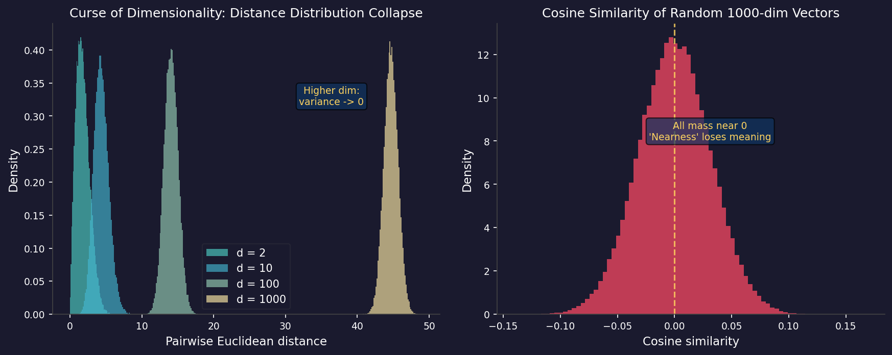
Figure 1: Left panel, distance distributions of random point pairs in 2, 10, 100, 1000 dimensions. The higher the dimension, the more concentrated the distribution, with variance tending to zero — "distance" loses its discriminative power. Right panel, histogram of pairwise cosine similarities of 1000-dimensional random vectors, almost entirely piled near zero.
This poses a fundamental problem for machine learning: if data were truly high-dimensional and random, then any algorithm based on distance or similarity — neural networks included — should not work.
But they do work.
There are two possible explanations here:
First, these algorithms bypass the constraints of high-dimensional geometry in some way we don't fully understand.
Second, the data itself is not high-dimensional random.
The second explanation is correct.
A Pause
Wait — don't rush to accept the conclusion that "the second explanation is correct."
Why would natural data cluster on a low-dimensional manifold? This is a fact that needs explanation, not an axiom.
One answer is: physical laws constrain the space of possible states — variations of human faces are governed by bones, muscles, and the physics of lighting, so possible faces are far fewer than possible pixel combinations.
But this answer implicitly assumes: the world has regularities, and these regularities are low-dimensional.
What justifies this assumption? If the world's true regularities were high-dimensional and chaotic, the Manifold Hypothesis would collapse — and machine learning shouldn't work.
Then why does it indeed work? Is it because physical laws truly are low-dimensional, or because we have only tested it on "those problems where the Manifold Hypothesis holds"?
Set this question aside for now.
II. The Manifold Hypothesis: Constraints Create Curved Surfaces
The core statement of the Manifold Hypothesis is:
Natural data (images, language, sound), though living in high-dimensional space, actually clusters near a smooth, curved surface (a manifold) whose intrinsic dimensionality is far lower than the ambient dimensionality.
"Manifold" is a mathematical term meaning a topological structure that locally looks like Euclidean space. A two-dimensional surface embedded in three-dimensional space is a manifold — the Earth's surface is a manifold, the Möbius strip is a manifold, the surface of a bent pipe is a manifold.
Manifold: Understanding Through the Earth's Surface
A manifold is a geometric object defined as: locally it looks "flat" (like ordinary Euclidean plane), but globally it can be curved.
The best example: the Earth's surface. If you stand at any point on Earth and look only at a very small patch under your feet, it looks no different from flat ground — this is "locally like Euclidean space." But globally, the Earth's surface is spherical, not flat. The Earth's surface is a 2-dimensional manifold embedded in 3-dimensional space.
In the machine learning context:
- The 49,152-dimensional space of face images = the analog of 3D space
- The few-dozen-dimensional curved surface where real face distributions live = the analog of the Earth's surface
Why is the Manifold Hypothesis important? Because it explains why machine learning can work: data is not high-dimensional random, but clusters on low-dimensional curved surfaces, and algorithms are actually learning the structure of this low-dimensional surface.
Let's build intuition with a concrete example:
A
But "real faces" occupy only an extremely tiny region of this space. What parameters determine a real face?
Identity (whose face)
Pose (how much the head is turned, at what elevation angle)
Lighting (where does the light come from, what intensity)
Expression (smiling? frowning?)
Age
About a dozen to a few dozen parameters can describe the vast majority of facial variations. This means the intrinsic dimensionality of face images is about a few dozen dimensions, not 49,152 dimensions.
Image data is squeezed onto a manifold of approximately a few dozen dimensions, embedded in 49,152-dimensional space.
The same is true for language data. "Grammatical English sentences" occupy only an extremely small fraction of all possible word sequences. "Semantically reasonable sentences" occupy an even smaller fraction of all grammatical English sentences. Each layer of constraint is a fold and a compression of the manifold.
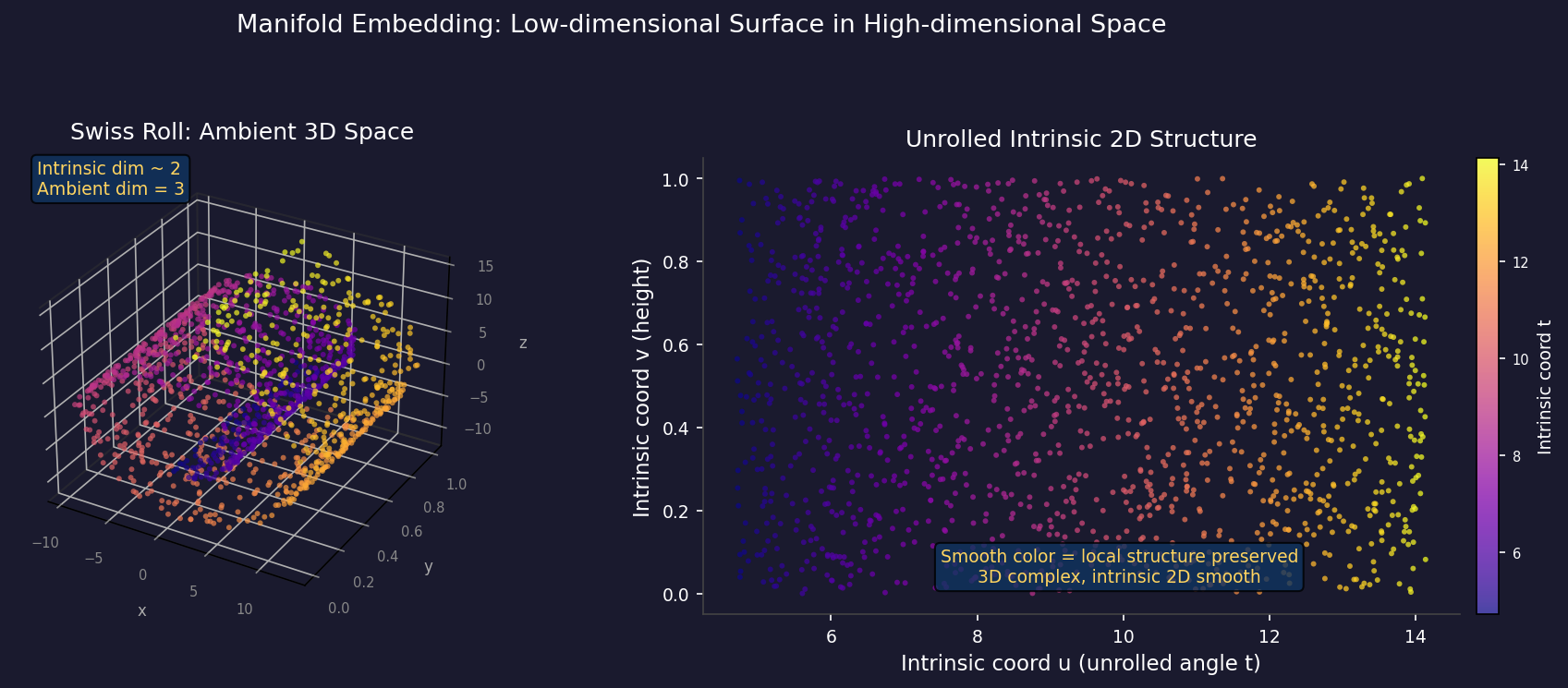
Figure 2: Left panel, a 2-dimensional manifold (Swiss Roll dataset) embedded in 3-dimensional space — the 3D coordinates appear complex, but the data is smoothly distributed along two intrinsic dimensions (u, v coordinates after unrolling). Right panel, manifold learning (UMAP) applied to the same dataset, recovering the intrinsic 2D structure. Colors encode the continuity of intrinsic coordinates — points that are locally adjacent in high-dimensional space remain adjacent.
Why does natural data cluster on a manifold? This is not coincidence; it is an inevitable consequence of the generative process.
All data is produced by some generative process. Face images are produced by biological processes — DNA, bone structure, skin texture — these parameters are finite and vary continuously. Language is produced by grammatical rules and semantic constraints. Music is produced by physics (sound waves) and cultural conventions.
The constraints of the generative process are the curvature of the manifold. The stronger the constraints, the lower-dimensional and more curved the manifold.
This is a profound fact: the intrinsic dimensionality of data is not an inherent property of the data, but a projection of the structure of the world that generates the data.
III. Training Is Folding
Now we arrive at the most important part of this chapter.
We usually say that neural networks are "learning" — learning to recognize cats, learning to translate languages, learning to predict the next word. This phrasing is dangerous. "Learning" implies some kind of understanding, some process of internalizing knowledge.
A more accurate phrasing is: neural networks are doing manifold transformations.
Let's unfold the working principle of an autoencoder:
where
What is happening here? The encoder
In other words, what the encoder learns is the parameterization of the manifold — it finds a set of coordinates that can be used to describe points on the manifold. What the decoder learns is the mapping between this set of coordinates and the original high-dimensional representation.
It's not just autoencoders. Classification networks do the same thing. When you train a ResNet to recognize image categories, the feature vector before the last fully connected layer is the manifold coordinates learned by the network — it's just that this coordinate system is specifically designed to be "useful for classification."
Backpropagation is the process of adjusting this coordinate system. Every gradient update changes the way the network maps high-dimensional inputs to the low-dimensional latent space — that is, it changes the parameterization of the manifold.
The essence of training is folding the manifold structure of past seen data into the curvature of the parameters.
The word "folding" matters. Not "storing," not "memorizing" — folding. Training data is not stored item by item into the network — the network doesn't have enough parameters to store every sample of the training set. What happens is: the statistical structure of the data, the geometric features of the manifold the data lives on, are compressed into the configuration of network weights.
This is not learning. This is topological compression.
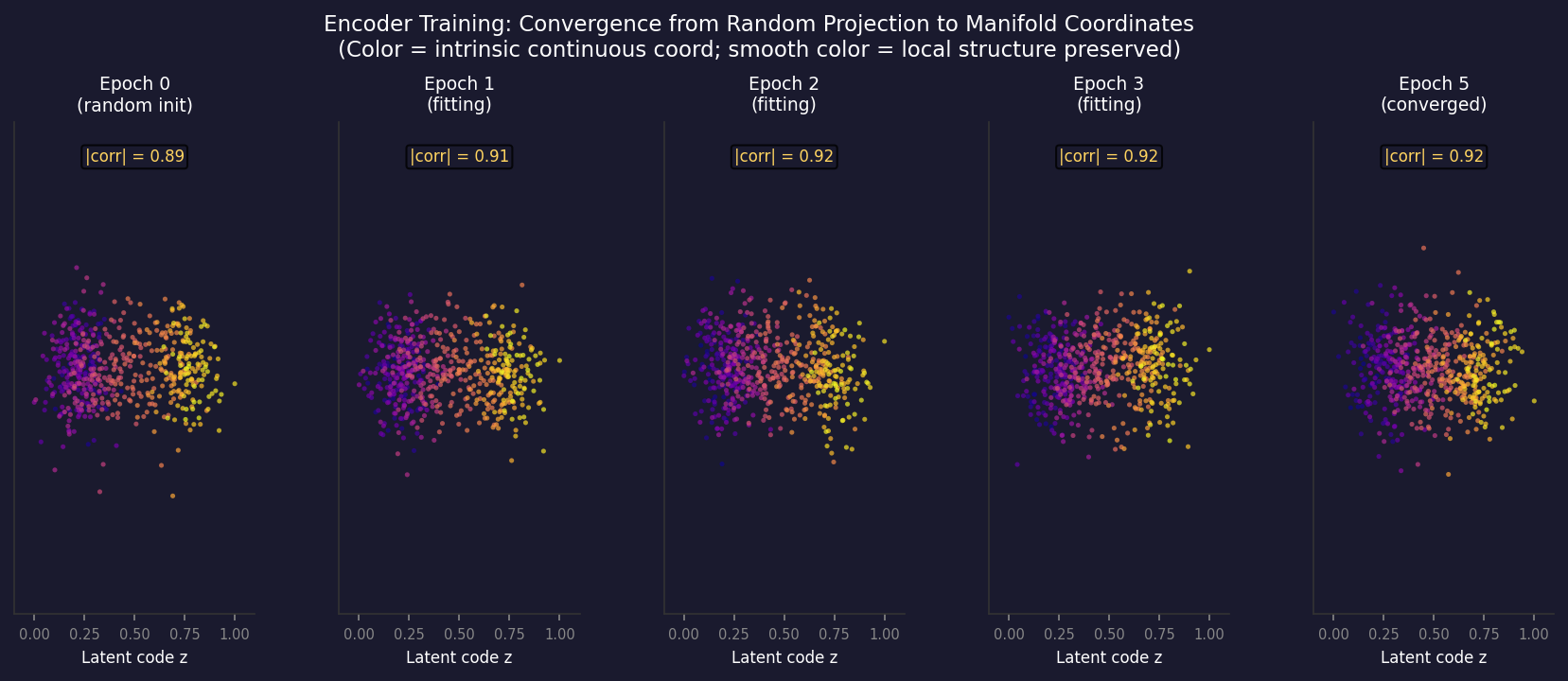
Figure 3: Top, the encoder progressively maps high-dimensional data (a 3D point cloud scattered on a 2D manifold) to 1D latent codes. Bottom, the evolution of the latent space during training — as epochs increase, the latent representation moves from chaotic to structured. Colors represent continuous coordinates of the data on the original manifold; color continuity means local structure is preserved.
Here is a deep question worth pausing to think about: What is stored in the parameters?
One intuition is: parameters store "knowledge" — about what cats look like, about grammatical rules, about physical laws.
But a more accurate formulation is: parameters store a compressed encoding of the manifold structure of the training data.
Knowing this, you can understand why pretraining is effective — the same manifold (e.g., "natural images") can be shared across multiple tasks, and the manifold parameterization learned in pretraining can be transferred.
You can also understand why fine-tuning sometimes changes model behavior and sometimes doesn't — it depends on whether the manifold on which your new task lives is a subset of the pretraining manifold.
And, you start to understand why large models hallucinate — about this, Act IV will discuss.
IV. The Bill for Compression
Any compression has a cost. This is not an empirical observation; it's an information-theoretic theorem.
Shannon's source coding theorem tells us: the limit of what you can losslessly compress is the entropy of the source. Beyond this limit, you must lose information. Neural network compression far exceeds this limit, so it must be losing information.
What is being lost?
The First Bill: Points off the Manifold
After training, the network's parameters encode the manifold on which the training data lives. When, at test time, it encounters a point not on this manifold — images from different distributions, unseen language phenomena, counterfactual reasoning scenarios — what does the network do?
It has no alert saying "this point is not on my manifold." It can only forcefully pull this point to the nearest region of the manifold, and then output an answer according to the logic of that region.
The result: confident error. Not "I don't know," but "it looks like X, so I answer X" — even if X is completely wrong.
This is the geometric root of the Distribution Shift problem: the manifold learned by the model and the manifold of the real world diverge outside the training distribution. The greater the shift, the greater the error, but the confidence remains unchanged — because confidence is a function of manifold coordinates, not a function of "how far from the manifold."
The Second Bill: Isometry Within the Manifold
During compression, certain regions of the manifold are "stretched," and certain regions are "compressed."
Where training data is dense, the network-learned parameterization has high resolution — adjacent inputs map to adjacent latent codes, and local geometry is well-preserved.
Where training data is sparse, the network parameterization has low resolution — adjacent inputs may be mapped far apart in latent space, or inputs far apart may be mapped to adjacent positions in latent space.
This means that the network generalizes well in dense regions of training data, and poorly in sparse regions — not randomly poor, but systematically poor: the manifold structure of sparse regions is "filled in by interpolation," padded with the most common patterns from the training data, not the true structure of that region.
The result of interpolation-based filling is hallucination.
The Third Bill: Tishby's Information Bottleneck
In 2017, Naftali Tishby proposed a theoretical framework for this process — the Information Bottleneck.
Training a neural network is essentially making a trade-off:
where
The first term
The second term
The optimal solution of this trade-off is a "sufficient statistic" — retaining all the information needed to predict the label while discarding all redundant information.
Tishby's claim is: the training process occurs in two phases — first the "fitting" phase, where mutual information
This theory is beautiful. But it is also controversial — subsequent work (Saxe et al., 2018) found that the compression phase does not appear in many situations, depending on the choice of activation function. The Information Bottleneck is a valuable analytical framework, but not a complete theory -> [Tishby & Schwartz-Ziv, 2017, arXiv:1703.00810] -> [Saxe et al., 2018, arXiv:1812.09881].
The Final Bill
Adding up the three bills, the cost of manifold compression is:
In-distribution: good generalization, accurate confidence
Distribution boundary: generalization begins to degrade, confidence remains high (danger zone)
Out-of-distribution: poor generalization, but confidence can still be very high (most dangerous zone)
The network does not know it is standing at the edge of the manifold. It only knows that the current input maps to some coordinate in latent space, and then outputs according to the logic of that coordinate. There is no built-in "uncertainty sensor" telling it: you are making an inference about a region you have never truly understood.
This is not a bug; it is an inevitable structural consequence of manifold compression.
V. The Limits of Compression: How Small Can a Manifold Be Compressed?
The Manifold Hypothesis says high-dimensional data is squeezed onto a low-dimensional manifold. So how "low" is this low dimension? To what extent can it be compressed?
This is an information-theoretic question, not merely a geometric one.
Rate-Distortion Theory Gives a Lower Bound
Shannon's rate-distortion theory tells us: to reconstruct a signal with distortion
For data on a manifold:
When you compress a neural network's hidden layer dimension from
Intrinsic Dimensionality
The intrinsic dimensionality of a manifold is the minimum number of coordinates needed to describe the manifold. This quantity can be estimated using the distribution of pairwise distances:
where
Experimental results are striking: the intrinsic dimensionality of ImageNet images is about 40, far lower than the raw pixel dimensionality (
This shows that real-world data is indeed squeezed onto extremely low-dimensional manifolds.
But a Hard Lower Bound Exists
Compression is not infinite. Once compressed below the intrinsic dimensionality, distortion rises sharply — you start losing the structure of the manifold itself, not merely losing noise.
This is why knowledge distillation (compressing from a large model to a small model) has a performance cliff: beyond a certain compression ratio, the model is not "a bit worse" but "completely collapses." The rate-distortion curve drops sharply after the inflection point.
This hard lower bound, and how to use randomization to break the limits of deterministic compression, is the topic of Chapter 11.
VI. A Brief Pause
Let me sort out what this chapter has done.
In high-dimensional space, random data cannot be learned — distance loses meaning, and sampling requires an exponential amount of data. The reason machine learning works is not that it has overcome high dimensionality, but that the data itself is not high-dimensional random. Natural data clusters on a low-dimensional manifold, a result of the combined action of the physical processes, biological constraints, and grammatical rules that generate the data.
The training of neural networks is the process of compressing the manifold structure of the training data into parameters. Not storage — compression. The compression ratio is on the order of 100:1 to 1000:1.
Compression has unavoidable costs: points off the manifold are forcibly projected, the structure of sparse regions is filled in by interpolation, and confidence decouples from accuracy under distribution shift. These costs are not engineering flaws; they are structural consequences of information-theoretic constraints.
This leads to the question of Chapter 5: if what models learn is manifold structure, not causal laws, then why do their out-of-distribution behaviors always fail systematically? What exactly is the gap between statistical correlation and genuine reasoning?
The manifold tells us where the data is, but it doesn't tell us whether what the model learns is the true law. In the next chapter, we will see how statistical fitting becomes a trap for reasoning.
Unresolved
How well does the manifold learned by a neural network "match" the manifold of real-world data? We lack good tools to measure this degree of match.
Can the intrinsic dimensionality of a manifold be estimated? What methods exist, and what assumptions do they each make? What is the intrinsic dimensionality in the activation space of LLMs?
Does the portion of information lost by "compression" contain the structures needed for reasoning? Or does reasoning ability happen to reside in the portion that is preserved?
If you train a neural network on completely random data, what kind of "manifold" would it learn? The answer to this thought experiment will tell us about the necessity of the Manifold Hypothesis.
The two-phase theory of the Information Bottleneck (fitting + compression) remains experimentally controversial. If the compression phase does not exist, what accounts for the generalization of neural networks?
The manifold structure of knowledge: Knowledge graphs are discrete symbolic manifolds; word vectors are continuous semantic manifolds. How do these two types of manifolds map onto each other and validate each other? Is there a unified "knowledge manifold" theory?
Multi-level manifolds: The phase-space manifold of physical systems (life), the logical-space manifold of symbolic systems (knowledge), the representation-space manifold of statistical systems (learning) — do there exist isomorphisms or mappings among these manifolds at different levels?
Try It Yourself: Compress a Manifold, Then Find Its Bill
The core proposition of this chapter is: compression has a cost, and the location of the cost is not random; it follows patterns. You will verify this firsthand using a minimal autoencoder — not to obtain a good model, but to precisely locate where compression lies.
Step 1: Generate Your Manifold Data
Don't use a real dataset; that introduces too many confounders. Start from a manifold whose generative process you fully understand.
Generate one of the following datasets:
Option A: A 2D Torus Embedded in 3D
import numpy as np
import matplotlib.pyplot as plt

np.random.seed(42)
N = 2000  # Number of sample points

# Uniformly sample the torus's two angular parameters
t = np.random.uniform(0, 2 * np.pi, N)   # Angle around the main axis
phi = np.random.uniform(0, 2 * np.pi, N) # Angle around the tube cross-section

r = 3.0    # Major torus radius
tube = 1.0 # Tube radius

# Torus parametric equations: embedded in 3D space
x = (r + tube * np.cos(phi)) * np.cos(t)
y = (r + tube * np.cos(phi)) * np.sin(t)
z = tube * np.sin(phi)

# Add small Gaussian noise to simulate measurement error
noise_std = 0.05
x += np.random.normal(0, noise_std, N)
y += np.random.normal(0, noise_std, N)
z += np.random.normal(0, noise_std, N)

# Assemble into data matrix, shape=(N, 3)
data_torus = np.stack([x, y, z], axis=1)
# Save intrinsic coordinates for later coloring (t is the main angle, phi is the tube angle)
intrinsic_t = t
intrinsic_phi = phi

# Visualization (colored by t values)
fig = plt.figure(figsize=(8, 6))
ax = fig.add_subplot(111, projection='3d')
sc = ax.scatter(x, y, z, c=t, cmap='hsv', s=2, alpha=0.6)
plt.colorbar(sc, label='Intrinsic coordinate t')
ax.set_title('Torus manifold (Option A)')
plt.tight_layout()
plt.show()
Option B: Swiss Roll (the data illustrated in this chapter)
import numpy as np
import matplotlib.pyplot as plt
from sklearn.datasets import make_swiss_roll

np.random.seed(42)
N = 2000  # Number of sample points

# Use sklearn to generate the standard Swiss Roll
# t is the intrinsic coordinate (roll angle), z is the intrinsic coordinate in the height direction
data_swiss, t_swiss = make_swiss_roll(n_samples=N, noise=0.1, random_state=42)
# data_swiss shape=(N, 3), columns are x, y, z (3D embedding coordinates)

# Or manually generate (equivalent effect):
t_manual = np.random.uniform(1.5 * np.pi, 4.5 * np.pi, N)  # Roll angle
x_manual = t_manual * np.cos(t_manual)
z_manual = np.random.uniform(0, 1, N)                        # Height (second intrinsic dimension)
y_manual = t_manual * np.sin(t_manual)
# Add small Gaussian noise
x_manual += np.random.normal(0, 0.1, N)
y_manual += np.random.normal(0, 0.1, N)
z_manual += np.random.normal(0, 0.05, N)

# Visualize the manually generated Swiss Roll (colored by t values)
fig = plt.figure(figsize=(8, 6))
ax = fig.add_subplot(111, projection='3d')
sc = ax.scatter(x_manual, y_manual, z_manual, c=t_manual, cmap='viridis', s=2)
plt.colorbar(sc, label='Intrinsic coordinate t (roll angle)')
ax.set_title('Swiss Roll manifold (Option B)')
plt.tight_layout()
plt.show()

# Use the sklearn version going forward (more standard)
data = data_swiss          # 3D coordinates, shape=(N, 3)
intrinsic_t = t_swiss      # Intrinsic coordinate t, used for coloring
Option B has an intrinsic dimensionality of 2 (t and z), embedded in 3D space.
Your first question (answer before writing code): What is the "true intrinsic dimensionality" of this data? If you use PCA for dimensionality reduction, how many principal components do you think you need to retain to preserve how much variance? Write down your prediction, and compare it with the actual results later.
Step 2: Implement a Minimal Autoencoder
Architecture definition:
import numpy as np
import torch
import torch.nn as nn
import torch.optim as optim
from torch.utils.data import DataLoader, TensorDataset

# ── Autoencoder architecture definition ──────────────────────────────────────────
class Autoencoder(nn.Module):
    def __init__(self, bottleneck_dim):
        super().__init__()
        # Encoder: 3 -> 16 -> d (bottleneck dimension)
        self.encoder = nn.Sequential(
            nn.Linear(3, 16),      # Input is 3-dimensional (embedded data points)
            nn.ReLU(),             # Nonlinear activation
            nn.Linear(16, bottleneck_dim)  # Output d-dimensional latent code z
        )
        # Decoder: d -> 16 -> 3 (reconstruct original coordinates)
        self.decoder = nn.Sequential(
            nn.Linear(bottleneck_dim, 16),
            nn.ReLU(),
            nn.Linear(16, 3)       # Output 3-dimensional reconstruction
        )

    def forward(self, x):
        z = self.encoder(x)    # Encode
        x_hat = self.decoder(z)  # Decode
        return x_hat, z

# ── Training function ────────────────────────────────────────────────────
def train_autoencoder(data_tensor, bottleneck_dim, n_epochs=300, lr=1e-3):
    """
    Train an autoencoder until reconstruction error converges.
    Returns the trained model.
    """
    dataset = TensorDataset(data_tensor)
    loader = DataLoader(dataset, batch_size=256, shuffle=True)

    model = Autoencoder(bottleneck_dim)
    optimizer = optim.Adam(model.parameters(), lr=lr)
    loss_fn = nn.MSELoss()  # Loss function: Mean Squared Error (reconstruction error)

    for epoch in range(n_epochs):
        for (batch,) in loader:
            optimizer.zero_grad()
            x_hat, _ = model(batch)
            loss = loss_fn(x_hat, batch)  # Reconstruction error
            loss.backward()
            optimizer.step()

    return model

# ── Example: using Swiss Roll data, initially set bottleneck dimension d=2 ───────────────
# (Assume data has been generated in the previous step, shape=(N, 3))
data_tensor = torch.tensor(data, dtype=torch.float32)  # Convert to PyTorch tensor

# Train an autoencoder with bottleneck dimension d=2
model_d2 = train_autoencoder(data_tensor, bottleneck_dim=2)
print("d=2 autoencoder training complete")
Train until reconstruction error converges. No need to tune hyperparameters; the default settings will work.
Step 3: Systematically Vary the Bottleneck Dimension and Record the Bill
Train with d = 1, 2, 3, 4, 5 respectively, and for each d, record:
import matplotlib.pyplot as plt
import torch
import torch.nn as nn

# Split data into training and test sets (80% / 20%)
N = len(data_tensor)
split = int(0.8 * N)
train_data = data_tensor[:split]
test_data  = data_tensor[split:]

results = {}  # Store results for each bottleneck dimension

for d in [1, 2, 3, 4, 5]:
    # 1. Train autoencoder
    model = train_autoencoder(train_data, bottleneck_dim=d, n_epochs=300)
    model.eval()

    with torch.no_grad():
        # 2. Compute average reconstruction error (MSE) on the training set
        train_hat, train_z = model(train_data)
        train_mse = nn.MSELoss()(train_hat, train_data).item()

        # 3. Compute average reconstruction error on the test set
        test_hat, test_z = model(test_data)
        test_mse = nn.MSELoss()(test_hat, test_data).item()

    results[d] = {'train_mse': train_mse, 'test_mse': test_mse,
                  'train_z': train_z.numpy(), 'model': model}

    # 4. Visualize the latent space (colored by intrinsic coordinate t values)
    train_t = intrinsic_t[:split]  # Intrinsic coordinates corresponding to training set
    if d == 1:
        # d=1: latent space is a line, draw a 1D scatter plot
        fig, ax = plt.subplots(figsize=(8, 2))
        sc = ax.scatter(train_z.numpy()[:, 0],
                        np.zeros(len(train_z)),
                        c=train_t, cmap='viridis', s=5)
        plt.colorbar(sc, label='Intrinsic coordinate t')
        ax.set_title(f'd={d} Latent space (1D)')
    elif d == 2:
        # d=2: directly draw 2D scatter plot
        fig, ax = plt.subplots(figsize=(6, 5))
        sc = ax.scatter(train_z.numpy()[:, 0],
                        train_z.numpy()[:, 1],
                        c=train_t, cmap='viridis', s=5)
        plt.colorbar(sc, label='Intrinsic coordinate t')
        ax.set_title(f'd={d} Latent space (2D)')
    plt.tight_layout()
    plt.show()

    # 5. Randomly sample 20 points from latent space, decode, and plot in 3D
    with torch.no_grad():
        # Uniformly sample in latent space (using the range of training set latent codes)
        z_min = train_z.min(dim=0).values
        z_max = train_z.max(dim=0).values
        z_samples = torch.rand(20, d) * (z_max - z_min) + z_min
        decoded_samples = model.decoder(z_samples).numpy()

    fig = plt.figure(figsize=(7, 5))
    ax = fig.add_subplot(111, projection='3d')
    ax.scatter(data[:split, 0], data[:split, 1], data[:split, 2],
               c='lightblue', s=1, alpha=0.3, label='Training data')
    ax.scatter(decoded_samples[:, 0], decoded_samples[:, 1], decoded_samples[:, 2],
               c='red', s=50, zorder=5, label='Random decoded points')
    ax.set_title(f'd={d} Random decoding (randomly sampled latent points)')
    ax.legend()
    plt.tight_layout()
    plt.show()

    print(f"d={d}: Train MSE={train_mse:.4f}, Test MSE={test_mse:.4f}")

print("\nComparison across bottleneck dimensions:")
for d, r in results.items():
    print(f"  d={d}: Train MSE={r['train_mse']:.4f}, Test MSE={r['test_mse']:.4f}")
Your second question: When d=1, the encoder compresses a 2D manifold into 1D. What does it preserve? What does it lose? Does the arrangement of points in the latent space preserve the topological structure of the original manifold (e.g., the toroidal relationship of the circle)?
Your third question (core question): When d=2, if you color the points in the latent space using the original intrinsic coordinates (t and φ, or t and z), are the colors continuously graded? If yes, what does that indicate? If not, what does that indicate?
Step 4: Find the Behavior of Out-of-Distribution Points
Generate a batch of points that are not on your manifold — for example, random 3D Gaussian noise points.
Feed this batch of points into your autoencoder:
import torch
import torch.nn as nn
import numpy as np
import matplotlib.pyplot as plt

# Use the d=2 model for out-of-distribution testing
model = results[2]['model']
model.eval()

# Out-of-distribution data: sample 100 points from a standard 3D Gaussian
# Note: these points are scattered throughout the 3D space, not restricted to near the manifold
ood_data = torch.randn(100, 3)  # Standard normal, mean 0, variance 1

with torch.no_grad():
    # Pass through autoencoder reconstruction (encode -> decode)
    ood_reconstructed, ood_z = model(ood_data)

# Compute reconstruction error for each category of data
loss_fn = nn.MSELoss(reduction='none')  # Compute error per sample individually
with torch.no_grad():
    train_hat, _ = model(train_data)
    # Per-sample MSE on training data (averaged over three dimensions)
    train_errors = loss_fn(train_hat, train_data).mean(dim=1).numpy()
    # Per-sample MSE on OOD data
    ood_errors   = loss_fn(ood_reconstructed, ood_data).mean(dim=1).numpy()

# Compare reconstruction errors
print(f"Training set average reconstruction error: {train_errors.mean():.4f} ± {train_errors.std():.4f}")
print(f"OOD point average reconstruction error: {ood_errors.mean():.4f} ± {ood_errors.std():.4f}")

# Visualization: plot the reconstruction results of OOD points in 3D space
# Observe where they land (whether they are "pulled" near the manifold)
fig = plt.figure(figsize=(10, 5))

# Left panel: original OOD points
ax1 = fig.add_subplot(121, projection='3d')
ax1.scatter(data[:500, 0], data[:500, 1], data[:500, 2],
            c='lightblue', s=2, alpha=0.3, label='Training manifold')
ax1.scatter(ood_data[:, 0], ood_data[:, 1], ood_data[:, 2],
            c='red', s=30, label='OOD original points')
ax1.set_title('OOD original points (scattered in 3D space)')
ax1.legend(fontsize=8)

# Right panel: positions of OOD points after autoencoder reconstruction
ax2 = fig.add_subplot(122, projection='3d')
ax2.scatter(data[:500, 0], data[:500, 1], data[:500, 2],
            c='lightblue', s=2, alpha=0.3, label='Training manifold')
ax2.scatter(ood_reconstructed[:, 0].numpy(),
            ood_reconstructed[:, 1].numpy(),
            ood_reconstructed[:, 2].numpy(),
            c='orange', s=30, label='OOD reconstructed points')
ax2.set_title('OOD points after reconstruction — "pulled" near the manifold')
ax2.legend(fontsize=8)

plt.tight_layout()
plt.show()
Your fourth question: After passing through the autoencoder, where are the out-of-distribution points "pulled" to? Are their reconstruction results random, or do they systematically land in a certain region of the training manifold?
This is exactly what Section IV of this chapter described: "The network has no alert saying 'this point is not on my manifold.' It can only forcefully pull this point to the nearest region of the manifold." You have just witnessed this process firsthand.
Step 5: Estimate the Intrinsic Dimensionality of Your Manifold
Returning to Step 1, now perform a data-driven intrinsic dimensionality estimate:
import numpy as np
import matplotlib.pyplot as plt
from sklearn.decomposition import PCA

# Perform PCA on the training data (using numpy arrays, not tensors)
train_np = data[:split]  # shape=(N_train, 3)

pca = PCA()               # No limit on number of components; compute all
pca.fit(train_np)

# Variance ratio explained by each principal component
explained_ratio = pca.explained_variance_ratio_
# Cumulative explained variance curve
cumulative_ratio = np.cumsum(explained_ratio)

# Plot cumulative variance curve
fig, axes = plt.subplots(1, 2, figsize=(12, 5))

# Left panel: variance explained by each principal component
axes[0].bar(range(1, len(explained_ratio) + 1), explained_ratio, color='steelblue')
axes[0].set_xlabel('Principal component number')
axes[0].set_ylabel('Explained variance ratio')
axes[0].set_title('Variance explained by each principal component')

# Right panel: cumulative explained variance curve, find the "elbow"
axes[1].plot(range(1, len(cumulative_ratio) + 1), cumulative_ratio,
             marker='o', color='tomato')
axes[1].axhline(y=0.95, color='gray', linestyle='--', label='95% threshold')
axes[1].set_xlabel('Number of principal components')
axes[1].set_ylabel('Cumulative explained variance ratio')
axes[1].set_title('Cumulative variance curve (find the elbow)')
axes[1].legend()

plt.tight_layout()
plt.show()

# Find how many principal components are needed for cumulative explained variance ≥ 95%
n_components_95 = np.searchsorted(cumulative_ratio, 0.95) + 1
print(f"Number of principal components needed for cumulative explained variance ≥ 95%: {n_components_95}")
print(f"Explained variance by each principal component: {explained_ratio.round(4)}")
print(f"Cumulative explained variance: {cumulative_ratio.round(4)}")

# Compare with autoencoder results
print(f"\nPCA-estimated intrinsic dimensionality: {n_components_95}")
print("Autoencoder test MSE at each bottleneck dimension:")
for d, r in results.items():
    print(f"  d={d}: Test MSE={r['test_mse']:.4f}")
print("(The inflection point where MSE suddenly spikes corresponds to the autoencoder-estimated intrinsic dimensionality)")
Compare this number with the prediction you wrote down in Step 1.
Your fifth question: Does the intrinsic dimensionality estimated by your PCA match the "minimum lossless bottleneck dimension" you obtained from the autoencoder? If there is a discrepancy, what do you think accounts for it — PCA's linearity assumption, or the autoencoder's nonlinearity?
Verification Criteria
After completing these five steps, you should be able to answer the following three questions — and answer them using your own experimental data, not using the text of this chapter:
When compression goes below the intrinsic dimensionality of the manifold, what is the cost? Where does the cost appear?
How are out-of-distribution points "hallucinatorily processed" after passing through the autoencoder?
"Where training data is dense, generalization is good; where sparse, generalization is poor" — in your experiment, which part of the manifold corresponds to sparse regions? Is reconstruction error higher there?
If you do only one thing, do Step 4. That is the shortest experiment that will most intuitively help you understand how "hallucination" happens.
Summary: From Manifolds to Knowledge Structures — The Deep Connections of the First Four Chapters
As we close the first four chapters, let us review the path we have walked, and the deep connections between the new content in Chapters 1 and 2.
Three Levels of Reasoning Systems
The first four chapters actually describe reasoning systems at three different levels, which share a meta-pattern:
The Physical Level (New in Chapter 1): Living systems as open systems
- Achieve local entropy reduction through energy flow
- Maintain order at the cost of environmental entropy increase
- Dissipative structures: self-organization far from equilibrium
The Symbolic Level (New in Chapter 2): Knowledge systems as symbolic structures
- Achieve precise reasoning through logical rules
- Obtain interpretability at the cost of construction effort
- Knowledge graphs: the scaled implementation of symbolism
The Statistical Level (Chapters 3-4): Learning systems as statistical models
- Learn pattern recognition through data flow
- Obtain generalization ability at the cost of computational complexity
- Manifold Hypothesis: the low-dimensional structure of high-dimensional data
A Unified Perspective: Structure, Cost, Flow
These three levels share a unified framework:
| Dimension | Physical Level (Life) | Symbolic Level (Knowledge) | Statistical Level (Learning) |
|---|---|---|---|
| Core mechanism | Energy flow | Logical reasoning | Pattern recognition |
| Form of order | Physical structure ordered | Symbolic structure ordered | Representation space ordered |
| Maintenance cost | Environmental entropy increase | Construction cost | Computational complexity |
| External input | Energy/matter | Knowledge/rules | Data/samples |
| Structural assumption | Dissipative structures | Closed world | Manifold Hypothesis |
From Discrete to Continuous: The Evolution of Representation
The first four chapters also showcase the evolutionary trajectory of knowledge representation:
- Discrete symbols (Chapter 2): If-Then rules, knowledge graph triples
- Continuous vectors (Chapter 3): Word embeddings, semantic space
- Low-dimensional manifolds (Chapter 4): Intrinsic dimensionality, the intrinsic structure of data
Key insight: Knowledge graphs are discrete symbolic manifolds; word vectors are continuous semantic manifolds. Both attempt to capture the structure of the world, just using different mathematical languages.
The Meta-Question: Multi-Level Implementation of Reasoning
This leads to a meta-question: What is reasoning?
- The physical answer: Reasoning is the cognitive strategy by which life counters entropy increase
- The symbolic answer: Reasoning is the derivation of a symbolic system following logical rules
- The statistical answer: Reasoning is pattern matching by a statistical model on a manifold
These three answers are all correct, but all incomplete. True reasoning may be the synergy of all three:
- The physical level provides the existential foundation (why reasoning is needed)
- The symbolic level provides the precise framework (how to formalize reasoning)
- The statistical level provides the implementation mechanism (how to compute reasoning)
Reflection Questions: Where Are the Boundaries?
Each level has its own boundaries:
- Physical level: thermodynamic limits (Landauer's principle)
- Symbolic level: knowledge boundary (closed-world assumption)
- Statistical level: generalization boundary (Manifold Hypothesis)
The ultimate question: When an AI system "reasons," at which level is it operating? Or does genuine intelligence require integration across these levels?
Further Reading
Tishby, N. & Schwartz-Ziv, M. (2017). Opening the Black Box of Deep Neural Networks via Information — The deep learning version of Information Bottleneck theory, proposing the two-phase training hypothesis
-> [arXiv:1703.00810]Saxe, A. et al. (2018). On the Information Bottleneck Theory of Deep Learning — Criticism and revision of Tishby's Information Bottleneck theory, showing the compression phase depends on activation function choice
-> [arXiv:1812.09881]Fefferman, C., Mitter, S. & Narayanan, H. (2016). Testing the Manifold Hypothesis — Mathematical testing of the Manifold Hypothesis: when does it hold, when does it not
-> [arXiv:1204.1423]Bengio, Y., Courville, A. & Vincent, P. (2013). Representation Learning: A Review and New Perspectives — A review of representation learning, including the relationship between manifold learning and deep representations
-> [arXiv:1206.5538]Bellman, R. (1957). Dynamic Programming — The original source of the Curse of Dimensionality; Bellman named this phenomenon in the context of optimization
[Zixi Li, 2026b] Collins — Randomized optimizer,
state compression, information-theoretic proof of safe compression ratio