Chapter 8: The Contract of Heuristics: How Much Courage Does It Take to Accept "Close Enough"?

If A*'s heuristic function lies, it will still give you a path. It's just that the path will be wrong.

---

I. The 1968 Wager

In 1968, Peter Hart, Nils Nilsson, and Bertram Raphael of the Stanford Research Institute proposed an algorithm in a paper that would later prove to be one of the most elegant ideas in the history of artificial intelligence.

The problem they wanted to solve was simple: let the robot Shakey find the shortest path from point A to point B in a room.

Brute-force search can guarantee finding the optimal solution—try all possible paths and pick the shortest one. But Shakey's world has millions of possible path combinations, and brute-force search requires an astronomical amount of time.

Greedy search is fast—always move toward the target direction. But it will crash into obstacles, walk into dead ends, and the path it finds may be much longer than the optimal solution.

The A* algorithm proposed by Hart and his two colleagues made a seemingly impossible promise: I can be orders of magnitude faster than brute-force search, while still guaranteeing finding the optimal solution.

What is the price of this promise? A contract.

If you give A* an "honest" heuristic function—one that never overestimates the remaining cost—it will keep its promise. But if the heuristic function "lies," overestimating the remaining cost, A* will still give you a path. It's just that the path may be wrong.

This is not a bug in the algorithm; it is its design. A* uses a mathematical contract to exchange for a balance between speed and optimality.

Over fifty years later, the idea of this contract remains at the core of heuristic algorithms: when perfection is unattainable, we need approximations with clearly defined costs.

---

II. The Curse of Combinatorial Explosion

Let me first quantify the matter of "perfection unattainable."

In 2016, AlphaGo defeated Lee Sedol. The world marveled at AI's "intuition" and "creativity." But few people noticed a technical detail: behind every move AlphaGo made, Monte Carlo tree search explored millions of possibilities on the 19×19 board.

Not hundreds, not thousands, but millions.

Why so many? Because the state space of Go is approximately ${10}^{170}$—90 orders of magnitude more than the number of atoms in the universe (${10}^{80}$).

Even if you could search ${10}^9$ states per second (the limit of modern computers), exhaustively exploring all possibilities would require ${10}^{150}$ times the age of the universe.

This is not an engineering problem; this is physical impossibility.

Similar combinatorial explosions are everywhere:

• Traveling Salesman Problem: All possible routes for visiting n cities number $n!$. For 20 cities, that's $2.4\times {10}^{18}$ routes.

• Protein Folding: For a protein of 100 amino acids, with each amino acid having 3 main conformations, there are approximately $3^{100}\approx {10}^{47}$ possible folding configurations.

• Theorem Proving: In first-order logic, for a proof of length n, the number of possible inference steps grows exponentially with n.

This is the reason heuristics exist: when the optimal solution is unattainable, we need a "good enough" solution.

But how good is "good enough"? This is not a vague engineering question, but a precise mathematical one. Heuristic algorithms must obey certain contracts—if these contracts are violated, the "approximate solution" they provide may be completely wrong.

Let me return to 1968 and see how Hart, Nilsson, and Raphael designed this contract.

---

III. A*'s Mathematical Contract

Suppose you are in a maze, trying to get from start point S to end point G. Every step has a cost (such as time or distance). You want to find the path with the minimum cost.

Brute-force search (Dijkstra's algorithm) will try all possible paths, guaranteeing finding the optimal solution, but the time complexity is $O(b^d)$—where b is the branching factor and d is the depth of the solution. In complex mazes, this is exponential.

Dijkstra's Algorithm: The Brute-Force Guarantee of Shortest Paths

Dijkstra's algorithm is a shortest-path algorithm proposed by Dutch computer scientist Edsger Dijkstra in 1956. The idea is: starting from the origin, at each step select the unvisited node with the smallest currently known cost, expand its neighbors, and continue until reaching the destination.

• Guarantee: If all edge costs are non-negative, Dijkstra will certainly find the optimal (minimum-cost) path
• Cost: It explores all possible paths, without knowing "roughly which direction is correct," making it inefficient

Branching factor $b$: In a search tree, the average number of child nodes (available next steps) each node has. In a maze, it might be 4 (up, down, left, right); in Go, it's approximately 250.

Search depth $d$: The number of steps needed to reach the answer.

Combined, the search space is $b^d$—this is the mathematical source of combinatorial explosion. A* uses a heuristic function to "prune" the search, reducing the number of nodes that need to be explored, thereby greatly accelerating the search while preserving optimality.

Greedy search at each step chooses the direction that "looks closest to the goal," which is fast but may walk into dead ends. Worse, the path it finds may be several times longer than the optimal solution.

When the A* algorithm was proposed in 1968, it made a seemingly impossible promise: I can be faster than Dijkstra, while still guaranteeing finding the optimal solution.

Its core is an evaluation function:

$$f(n)=g(n)+h(n)$$

• $g(n)$: the actual cost from the start to node n (known, definite)

• $h(n)$: the estimated cost from n to the goal (unknown, guessed)

• $f(n)$: the total estimated cost of reaching the goal via n

A* at each step expands the node with the smallest $f(n)$—that is, the node with the smallest "actual cost + estimated remaining cost."

The intuition behind this design is simple: if you have already taken 10 steps to reach node n, and you estimate you still need 5 steps to reach the goal, then the total cost via n is approximately 15 steps. A* prioritizes exploring the path with the smallest total cost.

But there is a fatal question here: how do you estimate $h(n)$?

If $h(n)$ is estimated too high, A* will prematurely abandon the optimal path—it will think "this path is too expensive" and turn to explore suboptimal paths.

If $h(n)$ is estimated too low (e.g., $h(n)=0$), A* degenerates into Dijkstra's algorithm, exploring all directions and losing its speed advantage.

Hart, Nilsson, and Raphael proved a profound theorem: if the heuristic function satisfies admissibility, A* is guaranteed to find the optimal solution.

Definition of admissibility:

$$h(n)\le h^{\ast }(n)$$

where $h^{\ast }(n)$ is the true shortest cost from n to the goal.

In other words, the heuristic function must be optimistic—it must never overestimate the remaining cost. You may underestimate (this will slow down the search), but you must not overestimate (this will cause the search to find the wrong answer).

This is A*'s contract: give me an admissible heuristic function, and I guarantee finding the optimal solution. Violate the contract, and the guarantee is void.

Why is this contract effective? Let me illustrate with a concrete example.

---

IV. Hands-On: Seeing How the Contract Is Broken

Admissibility is not an abstract mathematical requirement. It is a necessary and sufficient condition for A* to find the optimal solution.

Let us verify this with our own hands.

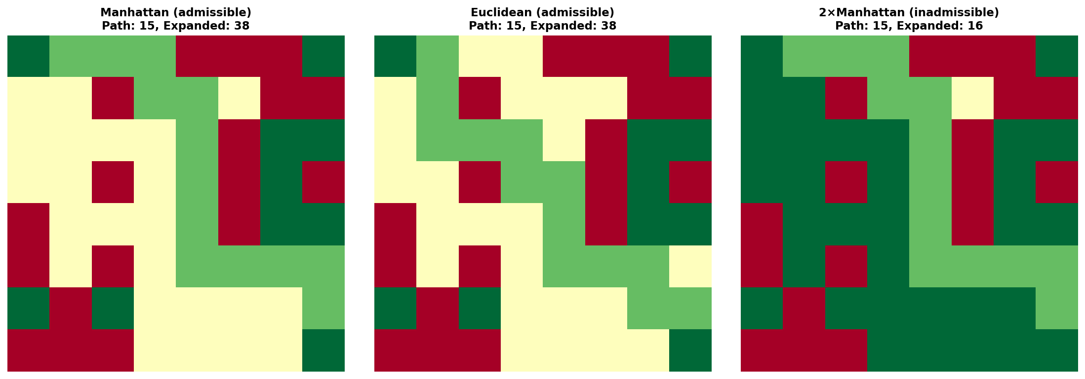
Experiment objective: Using the same maze, run A* with an admissible heuristic function and an inadmissible heuristic function respectively, and see how the results differ.

Maze map (0 = passable, 1 = obstacle, S = start, G = goal):

S . . . . .
. . . # . .
. . . . # .
. . . . . .
. . . . . #
. . . . . G

• S is the start point (0,0), G is the goal (5,5)

• . is a passable cell, cost per step = 1

• # is an obstacle, impassable

Task: Find the shortest path from S to G.

import heapq

# ------------------------------------------------------------------
# Define the maze: 6 rows, 6 cols, 1 = obstacle, 0 = passable
# S=(0,0), G=(5,5)
# ------------------------------------------------------------------
GRID = [
    [0, 0, 0, 0, 0, 0],  # row 0: S . . . . .
    [0, 0, 0, 1, 0, 0],  # row 1: . . . # . .
    [0, 0, 0, 0, 1, 0],  # row 2: . . . . # .
    [0, 0, 0, 0, 0, 0],  # row 3: . . . . . .
    [0, 0, 0, 0, 0, 1],  # row 4: . . . . . #
    [0, 0, 0, 0, 0, 0],  # row 5: . . . . . G
]
ROWS, COLS = len(GRID), len(GRID[0])
START = (0, 0)
GOAL  = (5, 5)

def neighbors(r, c):
    """Return the four (up/down/left/right) passable neighbors"""
    for dr, dc in [(-1,0),(1,0),(0,-1),(0,1)]:
        nr, nc = r+dr, c+dc
        if 0 <= nr < ROWS and 0 <= nc < COLS and GRID[nr][nc] == 0:
            yield nr, nc

def reconstruct_path(parent, node):
    """Backtrack from the parent dict to reconstruct the path"""
    path = []
    while node is not None:
        path.append(node)
        node = parent[node]
    return list(reversed(path))

def astar(h_func, label="A*"):
    """
    Generic A* search.
    h_func(r, c) is the heuristic function; returns (path length, path, number of expanded nodes).
    """
    # Priority queue elements: (f, g, node)
    open_heap = [(h_func(*START), 0, START)]
    g_cost = {START: 0}    # Actual cost from start to each node
    parent = {START: None} # Path backtracking
    closed = set()
    expanded = 0           # Count of expanded nodes

    while open_heap:
        f, g, node = heapq.heappop(open_heap)

        if node in closed:
            continue
        closed.add(node)
        expanded += 1

        # Reached goal
        if node == GOAL:
            path = reconstruct_path(parent, node)
            return len(path) - 1, path, expanded  # steps = nodes - 1

        # Expand neighbors
        for nb in neighbors(*node):
            new_g = g + 1  # cost per step = 1
            if nb not in g_cost or new_g < g_cost[nb]:
                g_cost[nb] = new_g
                parent[nb] = node
                f_val = new_g + h_func(*nb)
                heapq.heappush(open_heap, (f_val, new_g, nb))

    return None, [], expanded  # No solution

# ------------------------------------------------------------------
# Step 1: Admissible heuristic function — Manhattan distance
#   h₁(n) = |n_row - G_row| + |n_col - G_col|
#   Never overestimates remaining cost → satisfies admissibility → guarantees optimal solution
# ------------------------------------------------------------------
def h_admissible(r, c):
    """Manhattan distance: admissible, does not overestimate"""
    return abs(r - GOAL[0]) + abs(c - GOAL[1])

steps1, path1, exp1 = astar(h_admissible, "Admissible A*")
print("=== Step 1: Admissible heuristic (Manhattan distance) ===")
print(f"Path length: {steps1} steps")
print(f"Expanded nodes: {exp1}")
print(f"Path: {path1}")

# ------------------------------------------------------------------
# Step 2: Inadmissible heuristic function — Manhattan distance × 2
#   h₂(n) = 2 × (|n_row - G_row| + |n_col - G_col|)
#   Overestimates remaining cost → violates admissibility → may find suboptimal path
# ------------------------------------------------------------------
def h_inadmissible(r, c):
    """2× Manhattan distance: inadmissible, overestimates"""
    return 2 * (abs(r - GOAL[0]) + abs(c - GOAL[1]))

steps2, path2, exp2 = astar(h_inadmissible, "Inadmissible A*")
print("\n=== Step 2: Inadmissible heuristic (2× Manhattan distance) ===")
print(f"Path length: {steps2} steps")
print(f"Expanded nodes: {exp2}")
print(f"Path: {path2}")

# ------------------------------------------------------------------
# Comparison conclusion
# ------------------------------------------------------------------
print("\n=== Comparison Conclusion ===")
print(f"Admissible heuristic   → {steps1} steps (optimal solution guaranteed)")
print(f"Inadmissible heuristic → {steps2} steps ({'optimal' if steps1==steps2 else 'suboptimal, non-optimal'})")
if steps1 != steps2:
    print(f"  Gap: {steps2 - steps1} steps (contract was broken, a longer path was found)")
print(f"\nNote: Admissible version expanded {exp1} nodes, inadmissible version expanded {exp2} nodes.")
print("  The inadmissible heuristic expands fewer nodes, is faster, but sacrifices the optimality guarantee.")

Step 1: Using an Admissible Heuristic Function

The simplest admissible heuristic function is Manhattan Distance:

$$h_1(n)=|n_x-G_x|+|n_y-G_y|$$

This is the cost of "if there were no obstacles, walking in a straight line to the goal." Because the actual path must go around obstacles, $h_1(n)\le h^{\ast }(n)$, satisfying admissibility.

Starting from S, compute $f(n)=g(n)+h_1(n)$ for adjacent nodes:

Node	g(n)	h₁(n)	f(n)
S right	1	9	10
S down	1	9	10

Both tie at $f(n)$ (both 10), so A* chooses to expand S right. After moving along row 0 to the right to (0,2), two paths diverge: continue right along (0,3)→(0,4)→(0,5)→then south, or go down (1,2)→(2,2)→(2,3) through the gap. $h_1$ gives both paths equal opportunity—ultimately A* finds the optimal path through the gap, length = 10 steps, expanding a total of 33 nodes.

Step 2: Using an Inadmissible Heuristic Function

Now deliberately violate the contract. Define an overestimating heuristic function:

$$h_2(n)=2\times (|n_x-G_x|+|n_y-G_y|)$$

This function estimates the remaining cost as twice the Manhattan distance—clearly overestimating.

Restarting from S:

Node	g(n)	h₂(n)	f(n)
S right	1	18	19
S down	1	18	19

Both tie at $f(n)$ again, and A* similarly expands S right first. But $h_2$ has a key property: along any path heading toward the goal, each step makes $f_2=g+2h_1$ decrease by 1—$g$ increases by 1, $2h_1$ decreases by 2, net effect: $f_2$ gets smaller and smaller. The deeper you go, the "cheaper" it gets.

This creates a trap. After (0,2), at the fork:

• Right path: 5 consecutive steps straight to (0,5), $f_2$ decreasing at each step, like a snowball rolling faster and faster
• Gap path: down to (1,2), the right neighbor (1,3) is blocked by an obstacle, must go down one more level before turning right—needs one extra step to see progress

The decreasing effect of $f_2$ causes A* to irreversibly go all the way right along row 0. By the time it reaches (3,5) and discovers it needs to backtrack left to (3,4)—a step that makes the Manhattan distance rise instead of fall, causing $f_2$ to jump sharply—it is already too late. A* has already gone deep into this "increasingly cheaper" path, and the nodes on the gap side are all pressed to the bottom of the priority queue.

Result: The inadmissible $h_2(n)$ finds a path of length = 12 steps, 2 steps longer than the optimal solution. It expanded only 14 nodes—less than half of the admissible version (33)—but at the cost of losing optimality.

This failure is not accidental. A fundamental limitation of heuristic design is precisely this: you cannot reliably predict the behavior of a heuristic function before runtime. We tend to think that overestimating a little is merely "less accurate," but the $f_2$ decreasing effect systematically distorts the search direction—turning A* from a breadth-first, robust explorer into a snowballing, greedy gambler. With a different obstacle layout, it might fail or might not. That continuous overestimation actually expands fewer nodes than the admissible version—this in itself shows how hard heuristic behavior is to predict before runtime.

This is the meaning of admissibility: if $h(n)$ is admissible, the first path A* finds must be the shortest path. This is a mathematical guarantee, not an empirical regularity.

But admissibility also has a cost.

---

V. An Information-Theoretic Perspective: The Entropy Cost of Heuristic Functions

Admissibility guarantees correctness, but at what cost?

Consider two extremes:

Extremely conservative: $h(n)=0$, always estimating the remaining cost as 0.

This is clearly admissible (because the true cost $h^{\ast }(n)\ge 0$), but completely useless—A* degenerates into Dijkstra's algorithm, exploring uniformly in all directions until it bumps into the goal. From an information-theoretic perspective, this amounts to maximum-entropy exploration of the search space: every direction has equal prior probability.

Extremely aggressive: $h(n)=h^{\ast }(n)$, perfectly predicting the remaining cost.

This is the ideal case—A* would walk directly along the optimal path without exploring any useless nodes. This amounts to zero-entropy search: you already know the answer, no exploration needed. But the problem is: if you already know $h^{\ast }(n)$, you have already solved the problem and don't need to search.

Real-world heuristic functions lie between the two: as close as possible to $h^{\ast }(n)$, while remaining admissible.

This trade-off can be quantified using the effective branching factor $b^{\ast }$:

$$N=1+b^{\ast }+(b^{\ast }{)}^2+\cdots +(b^{\ast }{)}^d$$

where $N$ is the total number of nodes expanded by A*, and $d$ is the solution depth. The smaller $b^{\ast }$ is, the higher the search efficiency.

Pearl, in his classic 1984 textbook, provided experimental data:

• When $h(n)=0$, $b^{\ast }\approx 2.8$ (on the 8-puzzle)

• When $h(n)=\text{Manhattan distance}$, $b^{\ast }\approx 1.4$

• When using more precise heuristic functions (such as pattern databases), $b^{\ast }\approx 1.1$

Going from 2.8 down to 1.1 means the number of nodes in the search tree drops from ${2.8}^{20}\approx {10}^9$ to ${1.1}^{20}\approx 8$—a gap of six orders of magnitude.

The quality of the heuristic function directly determines the computational resources the search consumes.

But there is a deep tension here: a good heuristic function requires domain knowledge. Manhattan distance works for grids, but what about graph search? What about continuous spaces? What about Go?

In complex environments, designing a heuristic function that is both admissible and close to $h^{\ast }(n)$ is itself a difficult problem.

This is precisely the problem that \[Zixi Li, 2026a\]'s ADS work seeks to solve: can we let machines automatically learn heuristic functions?

---

VI. ADS: The Information-Theoretic Reformulation of Heuristics

Traditional heuristic design has a fundamental limitation: $h(n)$ is handcrafted, requires domain knowledge, and is static—once designed, it remains unchanged throughout the search process.

But the search space is dynamic. In open areas, the heuristic function is trustworthy; in obstacle-dense regions, any heuristic function may mislead. A fixed weight $\alpha =1$ is a crude simplification of this dynamic nature.

\[Zixi Li, 2026a\]'s ADS (Adaptive Dual Search) posed a question: can we use information theory to quantify the trustworthiness of the heuristic function, letting the weight adapt automatically to the uncertainty of the current state?

The core idea is to link the heuristic function's weight $\alpha$ to the entropy of the current state:

• When the model is highly certain about the current state (low entropy), $\alpha$ is large—trust the heuristic, advance quickly
• When the model is highly uncertain about the current state (high entropy), $\alpha \to \mathrm{\infty }$—forming a potential barrier that refuses entry into high-uncertainty regions

This is not parameter tuning, but rather quantifying uncertainty into an actionable search constraint. A*'s admissibility ensures "no overestimation"; ADS's entropy barrier ensures "no exploration of high-entropy dead ends."

Relationship to admissibility: Admissibility is a constraint on the value range of $h(n)$ (do not overestimate); ADS's entropy regularization is a constraint on the search direction (repel high uncertainty). The two are complementary: the former is static and mathematical; the latter is dynamic and information-theoretic.

The more complete technical details of ADS, and how it is applied to the LLM reasoning space, are unfolded in Chapter 10.

---

VII. The Contract of Approximation Algorithms: Abandoning Optimality, But Not Abandoning Guarantees

A*'s admissibility guarantees the optimal solution, but at the cost of having to explore all "potentially optimal" paths. On some problems, this is still too slow.

In 1973, the theory of computational complexity met a turning point. Stephen Cook proved that the SAT problem is NP-complete—if you can solve it in polynomial time, you can solve all NP problems.

This proof triggered a profound philosophical shift: perhaps we should give up seeking the optimal solution and instead seek a "good enough" solution.

But "good enough" needs a precise definition. Otherwise, any algorithm could claim to be "good enough."

In 1974, David Johnson introduced the concept of approximation ratio. For minimization problems, an α-approximation algorithm guarantees:

$$\text{algorithm solution}\le \alpha \times \text{optimal solution}$$

This is a worst-case guarantee—no matter the input, the approximation ratio will not exceed α.

Let me illustrate with a classic example.

7.1 Vertex Cover: A 2-Approximation Algorithm

Vertex Cover problem: Given a graph, find the smallest set of vertices such that every edge in the graph has at least one endpoint in the set.

This problem is NP-complete. Brute-force search requires checking $2^n$ possibilities (n is the number of vertices).

But there is an extremely simple 2-approximation algorithm:

import random

def greedy_vertex_cover(edges):
    """
    Greedy vertex cover: 2-approximation algorithm, time complexity O(|E|).
    edges: [(u, v), ...] list of edges
    Returns: vertex cover set C, guaranteeing |C| ≤ 2|C*|
    """
    remaining = list(edges)
    C = set()
    while remaining:
        u, v = random.choice(remaining)   # randomly pick an edge
        C.add(u)
        C.add(v)
        # Delete all edges connected to u or v
        remaining = [(a, b) for a, b in remaining if a not in (u, v) and b not in (u, v)]
    return C

The running time of this algorithm is $O(|E|)$ (E is the number of edges), and it guarantees:

$$|C|\le 2\times |C^{\ast }|$$

where $C^{\ast }$ is the optimal vertex cover.

Proof (this is a classic technique in approximation algorithm analysis):

For each edge $(u,v)$ selected, the optimal solution $C^{\ast }$ must contain at least one of u or v—otherwise this edge would not be covered.

Our algorithm selects both. So the number of vertices we select is at most twice the optimal solution.

This guarantee is tight—there exist inputs where the algorithm achieves exactly 2 times. But it is a worst-case guarantee: no matter the input, the approximation ratio will never exceed 2.

7.2 PTAS: Arbitrarily Close to Optimal

The holy grail of approximation algorithms is PTAS (Polynomial-Time Approximation Scheme).

A PTAS is a family of algorithms such that, for any $ϵ>0$, it can find a $(1+ϵ)$-approximate solution in polynomial time.

In other words, you can get arbitrarily close to the optimal solution—want 99% optimal? You can. Want 99.9% optimal? You can too. The cost is only a polynomial increase in time.

\[Li & Jin, 2015\] provided the first PTAS for the weighted unit disk cover problem. This problem has important applications in wireless network design: given points in the plane, cover all points with the minimum number of unit disks.

The time complexity of their algorithm is $O(n^{2/ϵ})$. Going from $ϵ=0.1$ to $ϵ=0.01$, the time grows from $O(n^{20})$ to $O(n^{200})$—still polynomial, but practically incomputable.

This reveals the limitation of PTAS: theoretically feasible, practically may be infeasible.

The contract of approximation algorithms: I do not guarantee giving you the optimal solution, but I guarantee the solution I give will not be too bad, and I can tell you precisely the degree to which it "won't be too bad." This is an honest contract—much stronger than "I tried my best."

---

VIII. Pseudocode: A* and Adaptive Heuristic Weights

Let me formalize the core algorithms discussed above.

Algorithm 1: Standard A* Search

import heapq

def astar(graph, start, goal, h):
    # graph: dict {node: [(neighbor, cost), ...]}
    # h: heuristic function h(node) -> estimated cost to goal
    # Returns: shortest path list, or None (no solution)
    open_heap = [(h(start), 0, start, [start])]  # (f, g, node, path)
    closed = set()

    while open_heap:
        f, g, node, path = heapq.heappop(open_heap)
        if node == goal:
            return path
        if node in closed:
            continue
        closed.add(node)
        for neighbor, cost in graph.get(node, []):
            if neighbor in closed:
                continue
            g_new = g + cost
            heapq.heappush(open_heap, (g_new + h(neighbor), g_new, neighbor, path + [neighbor]))

    return None  # No solution

Time complexity: $O(b^d)$, where $b$ is the branching factor and $d$ is the solution depth. The better the heuristic function, the fewer nodes are actually expanded.

Algorithm 2: ADS Adaptive Heuristic Weights

import math

def ads_search(start, goal, cost_fn, h_fn, policy_fn):
    # policy_fn(s) -> action probability distribution dict {action: prob}
    # h_fn(s)      -> heuristic estimate (cost to goal)
    # cost_fn(s,a) -> cost of executing action a
    def entropy(probs):
        return -sum(p * math.log(p + 1e-10) for p in probs if p > 0)

    s, path, g = start, [start], 0.0

    while s != goal:
        action_probs = policy_fn(s)
        actions = list(action_probs.keys())
        probs   = list(action_probs.values())

        U_s   = entropy(probs)
        H_max = math.log(len(actions) + 1e-10)

        # Logarithmic barrier: as B_s -> 1, alpha -> infinity, completely excluding high-entropy dead ends
        B_s   = U_s / (H_max + 1e-10)
        alpha = -math.log(1 - B_s + 1e-10)

        best_action, best_f = None, float("inf")
        for action in actions:
            f_val = g + cost_fn(s, action) + alpha * h_fn(action)
            if f_val < best_f:
                best_f, best_action = f_val, action

        g += cost_fn(s, best_action)
        s = best_action
        path.append(s)

    return path

Key innovation: α is not fixed, but dynamically adjusted based on the information-theoretic properties of the current state. When entropy is high (large uncertainty), reduce reliance on the heuristic; when entropy is low, trust the heuristic to advance quickly.

---

IX. Visualization: How Heuristic Weights Affect Search Paths

Imagine a 2D grid world with obstacles and a goal. Different heuristic weights α lead to completely different search behaviors.

Search behavior under three heuristic weight configurations: (a) α=0 (Dijkstra): uniform diffusion, exploring all directions, guaranteed optimal but inefficient. (b) α=1 (standard A): advancing along heuristic direction, moderate backtracking when encountering obstacles. (c) α=2 (greedy): over-trusting the heuristic, may fall into local optima. Green is the start, red is the goal, blue shading indicates expanded nodes, yellow line is the final path.*

Key observations: - α too small: search is too conservative, expanding many useless nodes - α too large: search is too aggressive, potentially missing the optimal path - α=1 with h admissible: the equilibrium point, guaranteeing optimality with high efficiency

The innovation of ADS lies in: α is not fixed, but adaptively adjusted based on local terrain.

This adaptivity comes from the computation of the information-theoretic barrier B(s): - In open areas: IG is high (large information gain along the heuristic direction), U is low (subsequent states are deterministic) → B is high → α is high - Near obstacles: IG is low (heuristic direction is blocked), U is high (multiple detour choices) → B is low → α is low

---

X. The Philosophy of Heuristics: The Courage to Accept Imperfection

Let me return to the question that opened this chapter: when perfection is unattainable, what should we do?

The answer from heuristic algorithms is: accept approximation with clearly defined costs.

This requires courage, because you must admit that perfection is unattainable. But this is not failure; it is wisdom.

Admissibility is A*'s contract: I may be optimistic, but I cannot lie. If $h(n)$ overestimates the cost, A* may find a suboptimal solution—the contract is broken, the guarantee is void. This is an honest contract: I tell you my assumptions; if the assumptions hold, I guarantee the result.

Approximation ratio is the contract of approximation algorithms: I do not promise optimality, but I promise not to be too bad. A 2-approximation algorithm guarantees that the solution does not exceed twice the optimal solution. This is a worst-case mathematical guarantee—not an average case, not "usually good," but "will never exceed 2 times."

Probabilistic guarantee is the contract of randomized algorithms: I do not guarantee correctness every time, but I guarantee correctness with probability $1-\delta$. This is a quantifiable risk: you can choose $\delta ={10}^{-6}$, making the failure probability less than one in a million.

These three contracts correspond to three different kinds of "imperfection":

1. Conditional guarantee: If the assumptions hold, I guarantee optimality (A*)

2. Worst-case guarantee: I guarantee not to be too bad, but may not be optimal (approximation algorithms)

3. Probabilistic guarantee: I am correct with high probability, but have a small probability of failure (randomized algorithms)

By contrast, contractless heuristics—"I tried my best," "usually good," "works on the data I tested"—are dishonest approximations. They do not tell you the conditions of failure, do not quantify the degree of "not good enough," do not give the probability of risk.

But heuristics also have costs:

Design cost: Good heuristic functions require domain knowledge. Manhattan distance works for grids, but what about graph search? What about continuous spaces? Every new problem requires redesigning the heuristic function.

Computational cost: A complex heuristic function may be slower than the search itself. If $h(n)$ requires $O(n^2)$ computation, you might as well search directly.

Generalization risk: A heuristic designed for a specific problem may fail when the scenario changes. This is why ADS uses neural networks to learn heuristic strategies—it can generalize across tasks. But the cost is the loss of mathematical guarantees.

This leads to a deep tension: provable guarantees vs. empirical generalization.

A* has admissibility guarantees, but requires handcrafted $h(n)$. Neural networks can learn automatically, but without guarantees. Can we have both?

This is the question of Chapter 12. For now, hold onto this tension.

---

XI. Yao's Principle: Algorithm Design as a Game

Before discussing how Collins breaks through deterministic lower bounds, we need to first understand a deeper question: who, exactly, is the adversary in heuristic design?

In 1977, Andrew Chi-Chih Yao, in a paper just a few pages long, gave an answer that changed the landscape of algorithmic complexity theory.

---

8.1 Turning Algorithm Design into a Game

Imagine a game like this.

There are two players:

• Player A (the algorithm designer): Chooses an algorithm $\mathcal{A}$ to solve some problem
• Player B (the adversary / input distribution): Chooses an input distribution $\mathcal{D}$, trying to make the algorithm run as slowly as possible

Does Player A move first or second? If A chooses the algorithm first, B constructs a worst-case input targeting that algorithm. If B chooses the distribution first, A optimizes the algorithm for that distribution.

This is a zero-sum game.

---

8.2 The Two Sides of the MiniMax Theorem

Yao's Minimax Principle says: Between deterministic algorithms and randomized inputs, there exists a MiniMax equality.

$$\underset{\text{deterministic algorithm}A}{min}\underset{\text{input distribution}\mathcal{D}}{max}{\mathbb{E}}_{x\sim \mathcal{D}}[T(A,x)]=\underset{\text{input distribution}\mathcal{D}}{max}\underset{\text{deterministic algorithm}A}{min}{\mathbb{E}}_{x\sim \mathcal{D}}[T(A,x)]$$

The left side of this equality is: "The expected time of the optimal deterministic algorithm under the worst-case input distribution."

The right side of this equality is: "The expected time of the optimal deterministic algorithm under some fixed input distribution."

The two sides are equal. This means: You can obtain a lower bound for all randomized algorithms by analyzing the lower bound of deterministic algorithms under a fixed distribution.

---

8.3 A Feynman-Style Explanation: Why Is This Profound?

Let me make this clear with an analogy.

Suppose you are a general (algorithm designer), trying to formulate a universal tactic (algorithm) to face different enemies (inputs). You don't know how the enemy will deploy.

Pessimistic scenario (MaxMin): You choose your tactic first, then the enemy chooses the deployment most unfavorable to you.

• Your optimal tactic = "The best result I can achieve under the worst enemy deployment"

Optimistic scenario (MinMax): The enemy chooses the distribution first, then you choose the best tactic.

• Your optimal tactic = "The best result I can achieve knowing the enemy's average deployment statistics"

The MiniMax theorem says: These two values are equal.

What does this mean?

The worst-case lower bound for deterministic algorithms = The average-case lower bound for randomized algorithms.

More bluntly: if you want to prove that "any deterministic algorithm requires at least $T$ steps," you only need to prove that "there exists some input distribution such that the expected time of any deterministic algorithm is at least $T$."

This is an extraordinarily powerful tool—you convert a "worst-case" analysis into an "average-case" analysis, and the latter is usually easier to handle.

---

8.4 A Game-Theoretic Perspective on Heuristic Design

Now apply this framework to heuristic design.

The design of the heuristic function $h(n)$ is, in essence, a game:

Player	Choice	Goal
Heuristic designer	Heuristic function $h(n)$	Minimize search time
Problem instance generator	Distribution of input graphs/mazes	Maximize search time

Yao's principle tells us: No matter how clever a deterministic heuristic is, there is a performance lower bound determined by the input distribution.

This lower bound is not an engineering limitation, but an information-theoretic limitation: if your heuristic function is deterministic, the adversary (input distribution) can always find a class of problems that degrades your performance to the worst case.

---

8.5 From Relative Lower Bounds to Absolute Lower Bounds

Here a critical distinction emerges:

Relative Lower Bound:

• "For the deterministic heuristic $h$, there exists an input such that the search time is $\mathrm{\Omega }(T)$"
• This is a lower bound relative to a specific algorithm—change the algorithm, and the lower bound may change

Absolute Lower Bound:

• "For any deterministic algorithm, the search time is $\mathrm{\Omega }(T)$"
• This is a lower bound about the problem itself—no deterministic algorithm can break it

Yao's principle builds a bridge between the two: through the game-theoretic MiniMax equality, you can elevate the worst-case lower bound of a specific algorithm into an absolute lower bound that holds for all deterministic algorithms.

But there is a trap here: this absolute lower bound only holds for deterministic algorithms.

Randomized algorithms are not subject to the same constraints.

Why? Because randomized algorithms break the symmetry of the game: the adversary cannot construct a worst-case input targeting a randomized algorithm—because the randomized algorithm runs differently each time, and the adversary does not know how to "target" it.

This brings us to Collins's core idea.

---

XII. Collins: Breaking Deterministic Lower Bounds with Randomization

Heuristics are typically deterministic: given state s, h(s) always returns the same value. But \[Zixi Li, 2026b\]'s Collins work shows that randomization can break through deterministic information-theoretic lower bounds.

Collins targets the optimizer state compression problem, but its core idea reveals a deep principle of heuristic design.

8.1 The Deterministic Information-Theoretic Lower Bound

Proposition 1 (Deterministic lower bound): Any deterministic data structure that maintains the state of d parameters with precision ε must use $\mathrm{\Omega }(d\log (1/ϵ))$ bits.

This is not an engineering limitation; this is an information-theoretic counting argument:

To distinguish $Q^d$ distinct states (where $Q=1/ϵ$ is the quantization level), you need at least ${\log }_2(Q^d)=d\log Q$ bits of information.

This means: if you want to use a deterministic method to store the first-order and second-order moments of the Adam optimizer (for d parameters), you need at least $O(d)$ memory.

For large language models (d can be in the billions), this is a massive bottleneck.

8.2 The Breakthrough of Randomization: Trading Probability for Space

Collins uses Count-Sketch + 2-Universal Hashing to reduce state complexity from $O(d)$ to $O(k)$, where $k\ll d$. The compression ratio $c=d/k$ can reach tens.

The key idea: do not store exact states, but store random projections of the states.

This is akin to coarse-graining in physics: you do not track the precise position of every particle, but track macroscopic statistics. The cost is introducing noise, but if the noise is sufficiently small, the macroscopic behavior remains correct.

The Chernoff bound gives a safety upper bound:

$$c_{\text{opt}}\le T_{\text{eff}}\cdot {\text{SNR}}_b$$

where $T_{\text{eff}}$ is the effective number of training steps, and ${\text{SNR}}_b$ is the batch signal-to-noise ratio.

Experiments verified the theoretical prediction: for $c\le 32$, convergence loss is indistinguishable from baseline; for $c>40$, there is sharp degradation—the phase transition point $c\approx 34$ is highly consistent with the theoretical prediction.

8.3 Implications for Heuristics: Deterministic vs. Probabilistic Guarantees

Collins's work reveals a deep trade-off in heuristic design:

Deterministic heuristics: Guarantee that for a given input, they always return the same estimate. But subject to information-theoretic lower bounds—a good heuristic function requires storing a large amount of domain knowledge.

Randomized heuristics: Trade probabilistic guarantees for lower computational/storage costs. Do not guarantee correctness every time, but guarantee "correct with high probability."

This is a different kind of contract—from "guaranteed correct" to "correct with probability $1-\delta$."

From a physics perspective, this is the manifestation of the Second Law of Thermodynamics: you can trade entropy (randomness) for energy (computational resources). Deterministic systems need to maintain a low-entropy state, at the cost of high energy consumption. Randomized systems permit higher entropy, so energy consumption is lower.

The Landauer principle gives the theoretical lower bound: erasing 1 bit of information requires at least $k_{B}T\ln 2$ of energy. Randomized heuristics do not erase information—they allow information to exist in the form of noise, so the energy cost is lower.

---

Heuristics perform approximation on known structures. In the next chapter, we will see how Transformers fundamentally reconstruct the concept of "structure" by dynamically connecting all nodes.

Unresolved Questions

• Can the "goodness" of a heuristic function be formally defined?

  What $h(n)$ is theoretically optimal? Pearl proved that consistency is stronger than admissibility, but is this the strongest useful condition? Does there exist "the admissible function closest to $h^{\ast }(n)$"? This question is equivalent to: given finite computational resources, how should they be optimally allocated to the design of the heuristic function?

• What is the boundary of applicability of the entropy barrier?

  ADS's dynamic logarithmic barrier works on arithmetic tasks but fails on abstract algebra. Is this failure principled or engineering? In other words: is entropy regularization itself unsuitable for high-order abstraction, or is it just that the 360M model is too small? If given a 3B model, would abstract algebra tasks succeed? This question touches on the fundamental limits of entropy as a reasoning constraint.

• What is the essential difference between implicit heuristics learned by neural networks and explicit heuristics designed by humans?

  AlphaGo's value network is a kind of heuristic function, but it does not satisfy admissibility—why does it still work? One possible answer: what the neural network learns is an average-case heuristic, while admissibility is a worst-case guarantee. But what does this mean? Does there exist a concept of "average-case admissibility"?

• What are the theoretical boundaries of randomized heuristics?

  Collins proved the deterministic lower bound $\mathrm{\Omega }(d\log (1/ϵ))$, but what is the upper bound for randomized approaches? The Chernoff bound gives $c_{\text{opt}}\le T_{\text{eff}}\cdot {\text{SNR}}_b$, but is this tight? Does there exist an "optimal randomized heuristic"—one that minimizes computational cost for a given failure probability $\delta$?

• Can heuristics learn online?

  Classical heuristics are designed offline—fixed before the search begins. But could we design a heuristic function that learns and adjusts itself during the search? Each time a node is expanded, update the estimate of $h^{\ast }(n)$, making subsequent search more efficient? This is similar to reinforcement learning, but the goal is to accelerate the current search, not to generalize to future tasks.

• Where are the lower bounds for approximation algorithms?

  We know vertex cover has a 2-approximation algorithm, but can we achieve 1.5-approximation? 1.1-approximation? For some NP-complete problems, there exist approximation lower bounds—unless P=NP, no $(1+ϵ)$-approximation algorithm exists. These lower bounds tell us: for some problems, even approximation is hard.

---

Extra Chapter: Search as Convergence—A Dynamical Systems Perspective on Heuristics

Every step of A* is, in fact, a Euler step.

Return to the evaluation function $f(n)=g(n)+h(n)$. View the search process as a discrete dynamical system in state space:

$$s_{t+1}=\arg \underset{a}{min}[g(s_t,a)+\alpha \cdot h(a)]$$

This has exactly the same structure as the Euler discretization of gradient descent:

$$x_{t+1}=x_t-\eta \mathrm{\nabla }E(x_t)$$

$g$ is the cost already incurred, the "past"; $h$ is the estimated remainder, the "future"; $\alpha$ is confidence in the future. Search is the process of approaching the goal step by step, pulled between these two forces.

What is a Euler step?

In calculus, the derivative describes continuous change. But computers can only do discrete things—each time, take a small step.

The Euler method divides "continuous flow" into small steps:

$$x_{t+1}=x_t+\mathrm{\Delta }t\cdot f(x_t)$$

Meaning: currently at $x_t$, rate of change is $f(x_t)$, take a small step $\mathrm{\Delta }t$, arrive at $x_{t+1}$.

Gradient descent is a special case of the Euler step—the direction of change is the negative gradient (steepest downhill direction), the step size is the learning rate $\eta$:

$$x_{t+1}=x_t-\eta \mathrm{\nabla }E(x_t)$$

A*'s search has the same structure: current state $s_t$, evaluate the cost in each direction, choose the smallest one and take one step. The only difference is that A* uses a discrete graph, while gradient descent uses a continuous surface. In essence, both are asking the same question: which direction should I go next to reach the goal as quickly as possible?

The triangle inequality is the guarantee of convergence.

The consistency condition $h(n)\le c(n,n^{\prime })+h(n^{\prime })$ is precisely the triangle relationship: $g$, $c$, $h$ form a triangle. This inequality guarantees that the $f$ value is monotonically non-decreasing—this is exactly the condition of a Lyapunov function: $V(s_{t+1})\le V(s_t)$, the system stably converges to the goal.

What is the triangle inequality?

You've known since elementary school: the sum of any two sides of a triangle is greater than the third side.

$a+b\ge c$

In heuristic search, this rule becomes: the estimated cost from $n$ to the goal cannot exceed the total cost of "first take one step to $n^{\prime }$, then from $n^{\prime }$ to the goal."

$$h(n)\le c(n,n^{\prime })+h(n^{\prime })$$

Intuition: your guess about the remaining distance cannot be more pessimistic than "guess again after actually taking one step." Otherwise, your map is self-contradictory—like a map claiming "Beijing to Shanghai: 2000 km, but Beijing to Nanjing: only 100 km, Nanjing to Shanghai: only 100 km." You would suspect it's lying.

A heuristic function satisfying this rule is called consistent. Consistency guarantees that A* will not backtrack, and each node only needs to be expanded once.

What is a Lyapunov function?

Imagine a ball rolling in a bowl. No matter where you release it, the ball will eventually roll to the bottom of the bowl.

The Lyapunov function is that "height of the bowl"—a numerical measure of how far the system is from the goal. As long as this value decreases (or does not increase) at each step, the system will certainly converge to the goal and won't wander off.

$$V(s_{t+1})\le V(s_t)$$

In A*, the $f$ value is this height of the bowl. Consistency guarantees $f$ is monotonically non-decreasing, which is equivalent to saying: we are always getting closer to the goal and will not go in circles.

Lyapunov used this idea in 1892 to prove the stability of a large class of dynamical systems. A*'s optimality proof is, in essence, the same thing.

What is ADS doing?

ADS's logarithmic barrier $\alpha =-\log (1-B_s)$ is dynamically deforming this triangle. When entropy is low, $\alpha \approx 0$, the triangle collapses, $g$ dominates; when entropy is high, $\alpha \to \mathrm{\infty }$, the $h$ side explodes, and high-uncertainty directions are completely excluded.

The barrier is not "tuning a parameter," but reshaping the geometry of the search space based on local uncertainty.

---

This "search as convergence" intuition is, in the context of heuristics, a geometric story.

But if we replace the search space with the LLM's belief space, replace $h$ with the cross-entropy energy function, and replace the Euler step with reasoning operators—the same convergence structure will have a deeper name.

To be revealed in Chapter 12.

---

Further Reading

• Hart, Nilsson, Raphael (1968). A Formal Basis for the Heuristic Determination of Minimum Cost Paths — The original A* algorithm paper, defining admissibility and consistency

• Yao, A. C.-C. (1977). Probabilistic Computations: Toward a Unified Measure of Complexity — The original paper on Yao's principle; the MiniMax theorem elevates deterministic lower bounds to randomized lower bounds → [FOCS 1977]

• \[Zixi Li, 2026a\] — ADS adaptive dual search, the information-theoretic reformulation of heuristics, knowledge distillation framework

• \[Zixi Li, 2026b\] — Collins randomized optimizer, deterministic lower bound and Chernoff upper bound, phase transition at $c_{\text{opt}}\approx 34$

• \[Li & Jin, 2015\] — PTAS for weighted unit disk cover, the gold standard of approximation algorithms → [arXiv:1502.04918]

• \[Esmer et al., 2022\] — Exponential-time approximation algorithms for approximate monotone local search → [arXiv:2206.13481]

• Pearl, J. (1984). Heuristics: Intelligent Search Strategies for Computer Problem Solving — The classic textbook on heuristic search

• Motwani, R. & Raghavan, P. (1995). Randomized Algorithms — The authoritative textbook on randomized algorithms published by Cambridge University Press, systematically covering Chernoff bounds, 2-Universal hashing, the MiniMax principle, and their applications in algorithm design

• Russell & Norvig (2020). Artificial Intelligence: A Modern Approach (4th ed.) — Chapters 3-4 discuss A* and its variants in detail