Chapter 6: The Boundary of Causality — Observational Data Is Never Enough

You have observed a thousand sunrises. Does that prove the sun will rise tomorrow? Hume says: No.

---

1. The Specter of Induction

In 1748, David Hume posed a disquieting question in An Enquiry Concerning Human Understanding:

On what grounds do we believe that the future will resemble the past?

The sun rises every day — that is a fact. We have observed a thousand, ten thousand sunrises. But does this prove that the sun will rise tomorrow?

Hume's answer is: No.

Logically speaking, there is no necessary deductive relationship between "the sun has risen every day in the past" and "the sun will rise tomorrow." You can imagine a world where the sun rises ten thousand times, and then stops on the ten-thousand-and-first — this imagination contains no logical contradiction.

This is the Problem of Induction: from finite observations, we cannot logically derive universal laws.

Hume's argument caused a massive upheaval in the history of philosophy, because it touches the foundations of the scientific method. Science relies on induction — deriving natural laws from experimental data. If induction is logically unreliable, what is the status of science?

Three hundred years later, this problem returned in a more technical form: From observational data, can we deduce causal relationships?

The answer is still: No.

What this chapter is about is the precise meaning of this "no," and how we can still make useful inferences within this limitation.

---

2. The Trap of Correlation

Let me start with a classic example.

In the 1950s, epidemiologists observed a strong statistical correlation: the incidence of lung cancer among smokers was significantly higher than among non-smokers.

Does this prove that smoking causes lung cancer?

The tobacco companies' lawyers said: No. They proposed an alternative explanation: perhaps there exists some hidden variable — such as a genotype — that simultaneously causes both "liking to smoke" and "being susceptible to lung cancer." Under this explanation, there is no causal relationship between smoking and lung cancer; they are merely two effects of a common cause.

Expressed as a causal diagram:

Hypothesis 1 (Causal):

Smoking → Lung Cancer

Hypothesis 2 (Confounded):

Genotype → Smoking
Genotype → Lung Cancer

In Hypothesis 2, the correlation between smoking and lung cancer is spurious — they are statistically correlated but have no direct causal link.

The key question is: Using only observational data, can you distinguish between these two hypotheses?

The answer is: No.

If genotype is unobservable (and in the 1950s it certainly was), then these two hypotheses make exactly the same predictions on all observational data. They are observationally equivalent.

This is not a problem of data quantity. You can observe a million samples — the correlation will become more significant, but you still cannot determine the causal direction — because observational data can only tell you the joint distribution of variables $P(X,Y)$, whereas causality is about intervention: if I forcibly change $X$, how will $Y$ change?

Observation and intervention are two different questions.

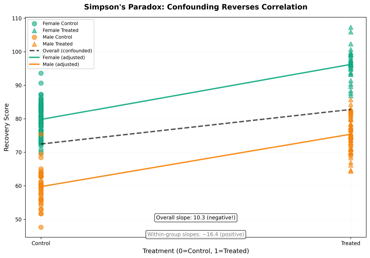
Figure 2: Geometric manifestation of Simpson's Paradox. The overall regression line (black dashed) has a negative slope — the treated group actually has a lower recovery rate. But after stratifying by gender, within females (blue line) and within males (red line), the treatment effect is positive. The confounding variable (gender) simultaneously affects treatment probability and baseline recovery rate, distorting the direction of the overall correlation. After backdoor adjustment eliminates confounding, the causal effect recovers the correct sign.

---

3. Bayesian Networks: Probabilistic Clothing for Causality

Before discussing Pearl's theory of causality, we need to understand Bayesian networks — because they are both the predecessor of Structural Causal Models, and their trap.

A Bayesian Network is a Directed Acyclic Graph (DAG) where nodes are random variables and edges represent conditional dependence relationships.

Bayesian Networks and DAGs: what does probability on a graph mean?

Directed Acyclic Graph (DAG): A graph is a set of nodes and the edges connecting them. "Directed" means each edge has a direction (A→B is different from B→A). "Acyclic" means following the edges, you can never return to the starting point.

Bayesian Networks are structures annotated with probabilities on a DAG:

• Each node is a random variable (e.g., "whether it rains," "whether to bring an umbrella")
• A directed edge A→B means "A has a conditional influence on B" — knowing the value of A changes our probability estimate for B

Key concept — Conditional Dependence: If, given the value of A, B and C become independent (no longer affect each other), then A is a "separating point" for B and C. Bayesian networks exploit these conditional independencies to decompose complex joint probabilities into products of smaller local probabilities, greatly reducing computation.

Important Warning: The edges in a Bayesian network represent statistical dependence, not necessarily causality — this is precisely the trap this section is about.

Given a Bayesian network $G=(V,E)$, the joint probability distribution can be factorized as:

$$P(X_1,\dots ,X_n)=\prod _{i=1}^{n}P(X_i\mid \text{Parents}(X_i))$$

This factorization has an elegant property: it decomposes a high-dimensional joint distribution into a product of a series of low-dimensional conditional distributions, greatly reducing the number of parameters that need to be estimated.

But there is a subtle point here: The edges of a Bayesian network are not necessarily causal relationships.

A Bayesian network is merely one way of factorizing a joint distribution. The same joint distribution can correspond to multiple different Bayesian networks — as long as they encode the same conditional independencies.

Consider an example. Three variables: $A$ (alarm sounds), $B$ (burglary), $E$ (earthquake).

The true causal structure is:

B → A ← E

A burglary or an earthquake can both trigger the alarm.

But from a purely probabilistic perspective, the following structure can also encode the same conditional independencies:

A → B, A → E

The alarm sounds, increasing the probability of both burglary and earthquake.

These two networks are equivalent on observational data — they correspond to the same joint distribution $P(A,B,E)$. But their causal meaning is completely different.

The first network says: intervening on $B$ (forcing a burglary) affects $A$ (the alarm sounds).

The second network says: intervening on $A$ (forcing the alarm to sound) affects $B$ (a burglary occurs) — which is obviously absurd; you cannot manufacture a burglary by pressing an alarm button.

Bayesian networks are probabilistic models, not causal models. Their edges represent conditional dependence, not causal flow.

Pearl's contribution was to add causal semantics on top of Bayesian networks — interpreting edges as causal relationships, and then defining what intervention and counterfactuals mean under this interpretation.

---

A Pause

The edges of a Bayesian network are not causal relationships — that alone is unsettling enough.

But there is an even deeper problem: even if you have Pearl's causal diagram, how do you know the diagram is correct?

The causal diagram itself is something you draw — it is your prior assumption about the structure of the world. Data can tell you which variables are conditionally independent, but that can only narrow down the set of possible causal diagrams — it cannot uniquely determine one.

This means: all conclusions of causal inference rest on an assumption that cannot be verified from the data — the diagram you drew.

If the diagram is wrong, the intervention effect computed by the do-operator is also wrong. You get an internally consistent but wrong answer.

So, on what grounds do we believe the causal diagram we drew? Experience? Intuition? Domain knowledge?

These are all answers, but none of them come from the data.

Let us set this question aside for now.

---

4. Pearl's Ladder of Causation

In his 2000 book Causality, Judea Pearl proposed a three-level framework for causal reasoning, later known as the Ladder of Causation.

The Ladder of Causation: Observation, Intervention, Counterfactual — three different kinds of questions

Pearl's Ladder of Causation divides "questions about causality" into three levels, each requiring stronger assumptions to answer:

Level 1 (Observation): Given that I see X, what is the probability of Y? A purely statistical question, requiring only data. Example: "Among smokers, what is the proportion with lung cancer?"

Level 2 (Intervention): If I forcibly make X happen, what is the probability of Y? Requires a causal diagram. Example: "If I made everyone smoke (random assignment), how much would the lung cancer rate change?" This is what randomized controlled trials (RCTs) do.

Level 3 (Counterfactual): If X had been different in the past, what would Y be now? Requires a complete structural causal model. Example: "This patient smoked and got lung cancer — if he had not smoked back then, would he still have gotten lung cancer?" This is a counterfactual inference about this specific individual, which cannot be directly answered by experiment.

Key Point: You cannot use information from a lower level to answer questions at a higher level. No amount of observational data can directly answer intervention or counterfactual questions — this is the precise meaning of "observational data is never enough."

Level 1: Association

Question form: $P(Y\mid X)$

"Given that I see $X$, what is the probability of $Y$?"

This is a purely statistical question. Given data, you can estimate conditional probabilities. The vast majority of machine learning tasks stay at this level: given features $X$, predict label $Y$.

Level 2: Intervention

Question form: $P(Y\mid do(X))$

"If I forcibly set the value of $X$, what is the probability of $Y$?"

Here $do(X)$ is the notation introduced by Pearl, representing an external intervention on $X$ — not observing $X$ occurring naturally, but forcibly setting $X$ to a certain value through some external operation.

$P(Y\mid do(X))$ and $P(Y\mid X)$ are usually different.

Let's give an example:

• $P(\text{Recovery}\mid \text{Taking medicine})$ may be high — because people with milder conditions are more likely to take medicine, and people with milder conditions are more likely to recover anyway.

• $P(\text{Recovery}\mid do(\text{Taking medicine}))$ is the true causal effect of the medicine — if we randomly assign who takes the medicine, what is the recovery rate in the medication group.

The first is observational, the second is interventional. Confusing the two is one of the most common errors in medical research.

Level 3: Counterfactual

Question form: $P(Y_x\mid X^{\prime },Y^{\prime })$

"If the value of $X$ in the past had been $x$ (instead of the actually observed $X^{\prime }$), then what would $Y$ be (given that we actually observe $Y^{\prime }$)?"

This is the hardest level, because it involves reasoning about things that did not happen.

Example:

• Observation: this patient took the medicine, and recovered.

• Counterfactual: if this patient had not taken the medicine, would he have recovered?

Counterfactual reasoning requires not just data, but also a structural causal model — mechanistic assumptions about how the world works.

Pearl's core argument is: These three levels cannot substitute for each other. You cannot use Level 1 information to answer Level 2 questions, nor can you use Level 2 information to answer Level 3 questions.

Each level requires stronger assumptions, more structure.

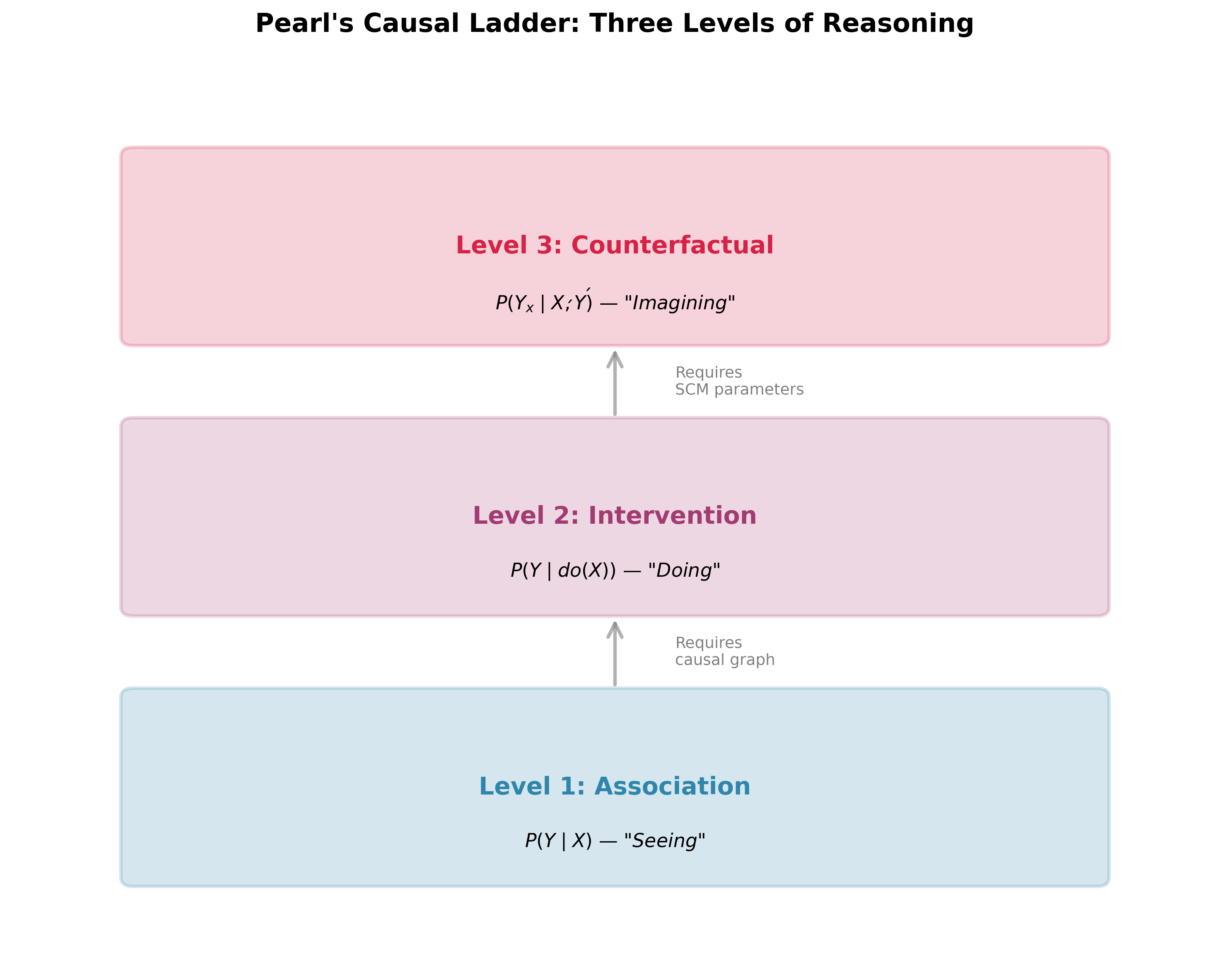
Figure 1: Pearl's Ladder of Causation. Level 1 (Observation) requires only data, answering "probability of Y given that I see X." Level 2 (Intervention) requires a causal diagram, answering "probability of Y given that I forcibly set X." Level 3 (Counterfactual) requires complete SCM parameters, answering "if X had been different in the past, what would Y be." Moving up each level requires stronger structural assumptions.

---

5. Structural Causal Models: The Blueprint of the World's Mechanisms

To answer intervention and counterfactual questions, we need a Structural Causal Model (SCM).

An SCM consists of three parts:

1. Endogenous Variables $V=\{V_1,\dots ,V_n\}$: the variables we care about

2. Exogenous Variables $U=\{U_1,\dots ,U_m\}$: external, unobservable random disturbances

3. Structural Equations $\mathcal{F}$: each endogenous variable is determined by a function

$$V_i=f_i(\text{Parents}(V_i),U_i)$$

Here $\text{Parents}(V_i)$ are the direct causes of $V_i$ (the nodes pointing to $V_i$ in the causal diagram), and $U_i$ is the exogenous noise affecting $V_i$.

Example: Smoking and Lung Cancer

Variables: - $S$: whether one smokes - $C$: whether one gets lung cancer - $G$: genotype (unobservable)

Structural equations:

G = U_G                    (genotype determined by exogenous factors)
S = f_S(G, U_S)            (smoking tendency influenced by genes and other factors)
C = f_C(S, G, U_C)         (lung cancer influenced by smoking, genes, and other factors)

Causal diagram:

G → S → C
G → C

This model encodes an assumption about the world: genotype $G$ simultaneously affects smoking tendency and lung cancer risk, while smoking $S$ also directly affects lung cancer $C$.

With an SCM, we can define intervention:

$$do(S=s)\text{ means: replace the structural equation }S=f_S(G,U_S)\text{ with the constant }s$$

The post-intervention model becomes:

G = U_G
S = s                      (forcibly set)
C = f_C(s, G, U_C)

Now $S$ no longer depends on $G$ — we have cut the edge $G\to S$. This is the graphical representation of intervention: delete all edges pointing into the intervened variable.

The post-intervention joint distribution $P(C\mid do(S=s))$ can be computed from the modified model.

Key point: $P(C\mid do(S=s))\ne P(C\mid S=s)$, because the latter includes the confounding effect of $G$ on both $S$ and $C$, while the former cuts off this confounding.

---

6. do-Calculus: The Bridge from Observation to Intervention

Now we arrive at a core question: Given observational data, can we compute the interventional distribution?

That is, can we derive $P(Y\mid do(X))$ (the interventional distribution) from $P(V)$ (the observational distribution)?

Pearl's do-calculus provides the answer: under certain conditions, yes.

do-calculus consists of three rules that allow you to manipulate probability expressions containing $do(\cdot )$ under the constraints of the causal diagram $G$.

Rule 1: Insertion/Deletion of Observations

$$P(Y\mid do(X),Z,W)=P(Y\mid do(X),W)\text{if }(Y\perp \perp Z\mid X,W{)}_{G_{\bar{X}}}$$

Where $G_{\bar{X}}$ denotes the graph after deleting all edges pointing into $X$.

Intuition: If, after intervening on $X$, $Z$ and $Y$ are conditionally independent (given $W$), then observing $Z$ provides no additional information.

Rule 2: Action/Observation Exchange

$$P(Y\mid do(X),do(Z),W)=P(Y\mid do(X),Z,W)\text{if }(Y\perp \perp Z\mid X,W{)}_{G_{\bar{X}\underset{―}{Z}}}$$

Where $G_{\bar{X}\underset{―}{Z}}$ denotes the graph after deleting edges into $X$ and deleting edges out of $Z$.

Intuition: If $Z$ does not affect $Y$ (after intervening on $X$), then intervening on $Z$ is equivalent to observing $Z$.

Rule 3: Insertion/Deletion of Actions

$$P(Y\mid do(X),do(Z),W)=P(Y\mid do(X),W)\text{if }(Y\perp \perp Z\mid X,W{)}_{G_{\bar{X}\overline{Z(W)}}}$$

Where $G_{\bar{X}\overline{Z(W)}}$ denotes the graph after deleting edges into $X$ and deleting edges into those nodes of $Z$ that are not ancestors of $W$.

Intuition: If $Z$ does not affect $Y$ (under a specific graph transformation), then the intervention on $Z$ can be ignored.

These three rules may look technical, but their power lies in this: they are complete.

Pearl and colleagues proved: if a causal effect $P(Y\mid do(X))$ can be identified from the observational distribution $P(V)$ and the causal diagram $G$, then the three rules of do-calculus are sufficient to derive it.

Conversely, if do-calculus cannot derive $P(Y\mid do(X))$, then it is unidentifiable — with only observational data and the graph structure, the causal effect cannot be determined.

---

7. The Backdoor Criterion and the Frontdoor Criterion

do-calculus is a theoretically complete tool, but in practice, we usually use more direct criteria to judge whether a causal effect is identifiable.

Backdoor Criterion

Given a causal diagram $G$, if there exists a set of variables $Z$ satisfying:

1. $Z$ blocks all backdoor paths from $X$ to $Y$ (paths that contain an edge pointing into $X$)

2. No element of $Z$ is a descendant of $X$

Then the causal effect can be computed via the adjustment formula:

$$P(Y\mid do(X))=\sum _{z}P(Y\mid X,Z=z)P(Z=z)$$

This is adjustment: eliminating spurious correlation by stratifying on the confounding variable $Z$.

Returning to the smoking and lung cancer example:

Causal diagram:

G → S → C
G → C

$G$ is a confounding variable on the backdoor path $S\leftarrow G\to C$. If we can observe $G$, then:

$$P(C\mid do(S))=\sum _{g}P(C\mid S,G=g)P(G=g)$$

This is why randomized controlled trials (RCTs) work: randomly assigning $S$ is equivalent to cutting $G\to S$, making $P(C\mid do(S))=P(C\mid S)$.

Frontdoor Criterion

But what if the confounding variable is unobservable?

Pearl discovered a clever situation: even if the confounding variable is unobservable, if there exists a mediator variable $M$ satisfying:

1. $M$ fully mediates the effect of $X$ on $Y$ ($X$ affects $Y$ only through $M$)

2. $X$ blocks all backdoor paths from $M$ to $Y$

3. All backdoor paths from $X$ to $M$ are blocked by the empty set

Then the causal effect can be computed via the frontdoor formula:

$$P(Y\mid do(X))=\sum _{m}P(M=m\mid X)\sum _{x^{\prime }}P(Y\mid M=m,X=x^{\prime })P(X=x^{\prime })$$

This formula does not require observing the confounding variable — it bypasses confounding through the mediator $M$.

Example: Smoking, Tar, Lung Cancer

U → S → T → C
U → C

$U$ is an unobservable confounder (e.g., genotype), $T$ is tar deposits (observable mediator).

Even if we cannot observe $U$, we can still compute $P(C\mid do(S))$ via the frontdoor criterion — because $T$ fully mediates the effect of $S$ on $C$.

This is a profound result: Under certain structures, observational data is sufficient to identify causal effects, even in the presence of unobservable confounding.

But "certain structures" is the key — not all causal diagrams satisfy the backdoor or frontdoor criteria.

8. Observational Equivalence Classes: The Indistinguishability of Causal Diagrams

Now we arrive at the most critical point of this chapter. Even if you have infinite observational data, you still cannot uniquely determine the causal diagram — because multiple different causal diagrams can produce the same observational distribution.
These diagrams are called Markov Equivalence Classes.
Definition: Two DAGs $G_1$ and $G_2$ are Markov equivalent if they encode the same conditional independence relations.
Equivalent diagrams have the same skeleton (the undirected graph obtained by ignoring edge directions) and the same v-structures (structures of the form $A\to C\leftarrow B$, where $A$ and $B$ are not adjacent).
Example: Equivalence Class of Three Variables
Consider three variables $X,Y,Z$. The following three diagrams are Markov equivalent:
X → Y → Z X ← Y → Z X ← Y ← Z
They all encode the same conditional independence: $X\perp \perp Z\mid Y$.
From observational data, you cannot distinguish these three diagrams — because they correspond to the same joint distribution.
But their causal meanings are completely different:

• First diagram: $X$ affects $Y$, $Y$ affects $Z$ - Second diagram: $Y$ affects both $X$ and $Z$ - Third diagram: $Z$ affects $Y$, $Y$ affects $X$
  If you want to know $P(Z\mid do(X))$, these three diagrams will give different answers.
  The Root of Unidentifiability
  This is not a problem of data quantity, nor of algorithms — it is a structural impossibility.
  Observational data can only tell you conditional independencies — which variables are independent given other variables. But causality is not just about independence; it is about behavior under intervention.
  Two diagrams can have the same observational distribution but behave completely differently under intervention.
  This means: With only observational data, causal discovery can only recover up to the Markov equivalence class, and cannot determine a unique causal diagram.
  To break the equivalence class, you need additional information:

1. Interventional data: If you can perform experiments, forcibly changing certain variables and observing the response of other variables, you can determine causal directions 2. Temporal order: If you know $X$ occurred before $Y$, then $Y\to X$ is impossible 3. Functional form assumptions: If you assume causal mechanisms are linear, or are additive noise models, certain equivalence classes can be broken 4. Prior knowledge: If you know that certain edges cannot exist (e.g., "age cannot be affected by income"), you can exclude certain diagrams
   But if you only have observational data, with no additional assumptions, the causal diagram is unidentifiable.

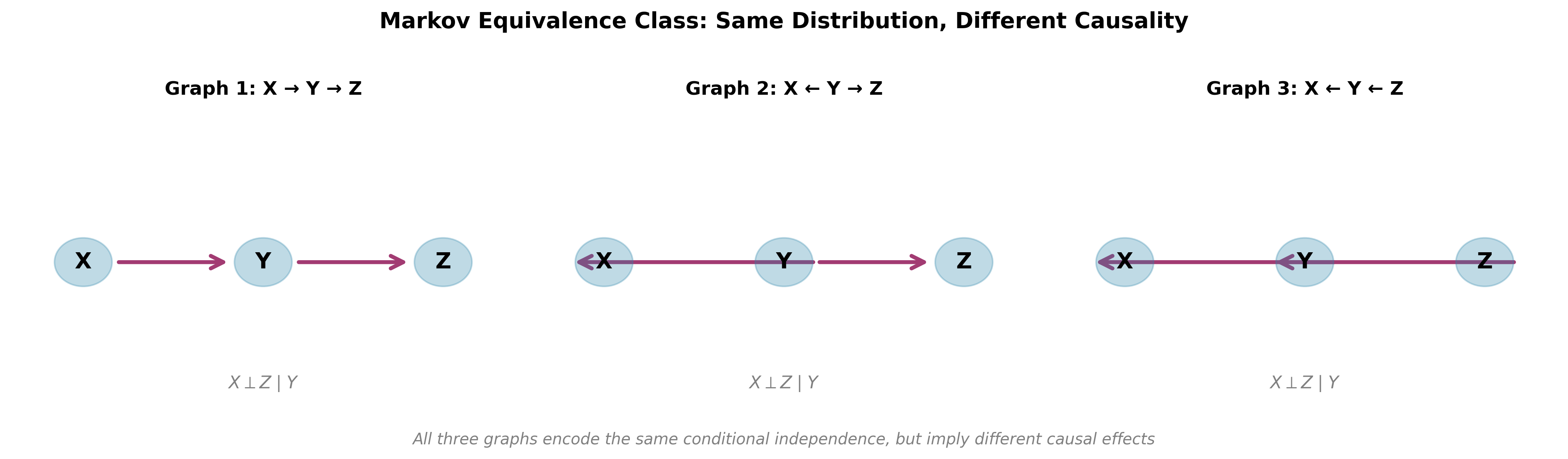
Figure 3: Markov Equivalence Class example. Three different causal diagrams (X→Y→Z, X←Y→Z, X←Y←Z) encode the same conditional independence X⊥⊥Y Z, and are therefore completely equivalent on observational data. But their causal meanings differ: in the first diagram, do(X) affects Z; in the second, it does not. Observational data alone cannot distinguish them.

9. The Faithfulness Assumption: A Fragile Bridge

Causal discovery algorithms (such as the PC algorithm and GES algorithm) typically rely on two assumptions:

Assumption 1: The Causal Markov Condition

Given its parents, each variable is independent of its non-descendants.

This is the standard assumption of Bayesian networks, and is usually reasonable.

Assumption 2: Faithfulness

All conditional independencies in the observational distribution are entailed by d-separation in the causal diagram.

In other words: if $X\perp \perp Y\mid Z$ holds in the data, then $X$ and $Y$ are d-separated by $Z$ in the diagram.

This assumption seems harmless, but it is actually quite strong.

Counterexample: Accidental Parameter Cancellation

Consider the following causal diagram and structural equations:

X → Y → Z
X → Z

Y = a·X + U_Y
Z = b·Y + c·X + U_Z

If the parameters happen to satisfy $b\cdot a+c=0$, then the total effect of $X$ on $Z$ is zero — the direct effect $c$ and the indirect effect through $Y$, $b\cdot a$, cancel each other out.

In this case, the observational data would show $X\perp \perp Z\mid Y$, but this is not because of the graph structure, but because of a coincidence of parameters.

The faithfulness assumption rules out such coincidences — it assumes parameters are in "general position" and do not accidentally cancel.

But in the real world, such coincidences may not be rare. Biological systems and economic systems contain numerous feedback and balancing mechanisms, whose parameters may happen to make certain effects cancel each other out.

Consequences of Faithfulness Failure

If faithfulness does not hold, causal discovery algorithms will infer incorrect graph structures — they will think certain edges are absent, because the corresponding variables appear independent in the data, but in fact they have a causal relationship, only the effect is canceled out.

This is a deep vulnerability: causal discovery relies on an assumption about parameters, and this assumption cannot be tested in the data — because you cannot distinguish "true independence" from "accidental cancellation."

---

10. Counterfactuals: The Hardest Level

The third level of Pearl's Ladder of Causation — counterfactuals — is the hardest, because it involves reasoning about things that did not happen.

Definition of Counterfactual

Given an SCM and observed evidence $X=x^{\prime },Y=y^{\prime }$, the counterfactual question is:

$$P(Y_x\mid X=x^{\prime },Y=y^{\prime })$$

"If the value of $X$ had been $x$ (instead of the actually observed $x^{\prime }$), then what would $Y$ be (given that we observe $Y=y^{\prime }$)?"

Computing counterfactuals requires three steps:

Step 1: Abduction

Update beliefs about the exogenous variables $U$ based on the observed evidence:

$$P(U\mid X=x^{\prime },Y=y^{\prime })$$

Step 2: Action

Modify the SCM, replacing the structural equation for $X$ with $X=x$ (intervention).

Step 3: Prediction

Under the modified model and the updated distribution of $U$, compute the distribution of $Y$:

$$P(Y_x\mid X=x^{\prime },Y=y^{\prime })=\sum _{u}P(Y_x\mid U=u)P(U=u\mid X=x^{\prime },Y=y^{\prime })$$

Example: Individual Causal Effect of a Drug

Suppose we have the following SCM:

X = U_X                    (whether the drug is taken, determined by exogenous factors)
Y = a·X + U_Y              (recovery status)

Observation: a certain patient took the drug ($X=1$) and recovered ($Y=1$).

Counterfactual question: if this patient had not taken the drug ($X=0$), would he have recovered?

Step 1: Infer $U_Y$ from $X=1,Y=1$:

$$1=a\cdot 1+U_Y⟹U_Y=1-a$$

Step 2: Intervene $X=0$.

Step 3: Compute the counterfactual outcome:

$$Y_0=a\cdot 0+U_Y=1-a$$

If $a>0$ (the drug has a positive effect), then $Y_0<1$ — this patient, had he not taken the drug, would have had a lower degree of recovery.

The Unidentifiability of Counterfactuals

Key issue: counterfactuals are typically unidentifiable.

Even if you know the causal diagram, even if you have infinite observational data, you still cannot uniquely determine the counterfactual distribution from the data — because counterfactuals depend on the distribution of exogenous variables $U$, and $U$ is unobservable.

In the example above, if we do not know the value of $a$ (the magnitude of the drug's effect), we cannot compute $Y_0$.

Counterfactuals require not just the causal diagram, but also parameterized structural equations — which is a stronger assumption than the graph structure alone.

This is why counterfactual reasoning is difficult in practice: it requires a complete, parameterized model of the world, and this model typically cannot be fully learned from data.

11. Pseudocode: Core Algorithms of Causal Inference

Let me formalize the core algorithms discussed above.

Algorithm 1: Backdoor Adjustment

import itertools
import numpy as np

def backdoor_adjustment(data, x_col, y_col, z_cols, x_val):
    """
    Backdoor adjustment to estimate causal effect P(Y | do(X=x_val)).
    data:    pandas DataFrame, containing observational data
    x_col:   name of the intervention variable column
    y_col:   name of the outcome variable column
    z_cols:  list of adjustment set column names (satisfying the backdoor criterion)
    x_val:   intervention value
    Returns: estimate of P(Y=1 | do(X=x_val))
    """
    if not z_cols:
        raise ValueError("Adjustment set is empty; causal effect is unidentifiable (via backdoor adjustment)")

    # Enumerate all value combinations of Z
    z_values = [data[z].unique() for z in z_cols]
    result = 0.0

    for z_combo in itertools.product(*z_values):
        # Conditional probability P(Y | X=x_val, Z=z_combo)
        mask_xz = (data[x_col] == x_val)
        for z_col, z_val in zip(z_cols, z_combo):
            mask_xz &= (data[z_col] == z_val)
        if mask_xz.sum() == 0:
            continue
        p_y_given_xz = data.loc[mask_xz, y_col].mean()

        # Marginal probability P(Z=z_combo)
        mask_z = np.ones(len(data), dtype=bool)
        for z_col, z_val in zip(z_cols, z_combo):
            mask_z &= (data[z_col] == z_val)
        p_z = mask_z.mean()

        result += p_y_given_xz * p_z

    return result

12. A Small Pause

Let me sort out what this chapter has done.

Hume's problem of induction returned three hundred years later in the form of causal inference: from observational data, can we deduce causal relationships? The answer is: No — at least not uniquely.

Observational data can only tell us the joint distribution of variables $P(X,Y)$, while causality is about intervention $P(Y\mid do(X))$. These two are usually different, because observation includes confounding effects.

Pearl's Ladder of Causation divides reasoning into three levels: observation, intervention, and counterfactual. Each level requires stronger assumptions. The vast majority of machine learning tasks stay at the first level, while genuine causal reasoning requires the second or third level.

Structural Causal Models (SCMs) provide a framework that uses structural equations and causal diagrams to encode the mechanisms of the world. With an SCM, we can define intervention (deleting edges pointing into the intervened variable) and counterfactuals (the three-step abduction-action-prediction method).

do-calculus provides complete rules for deriving interventional distributions from observational distributions. The backdoor criterion and frontdoor criterion are more direct tools in practice — under certain graph structures, observational data is sufficient to identify causal effects.

But the core limitations remain:

1. Markov Equivalence Classes: Multiple causal diagrams can produce the same observational distribution; observational data alone cannot distinguish them

2. The Faithfulness Assumption: Causal discovery relies on an assumption about parameters being in "general position," and this assumption cannot be tested in the data

3. The Unidentifiability of Counterfactuals: Counterfactual reasoning requires parameterized structural equations, not just the causal diagram

This leads to the question of Chapter 7: if observational data is not enough, what do we need? The answer is intervention — actively changing the world, rather than just passively observing it. Randomized controlled trials (RCTs) are the gold standard of causal inference, not because they are more precise, but because they break the prison of observation.

---

Causal inference reveals the limitations of observation. In the next chapter, we turn to another boundary — the asymmetry of computation itself: why is finding an answer so much harder than verifying one?

Unresolved

• How often does the faithfulness assumption fail in the real world? Do we have methods to detect faithfulness failures?

• If two causal diagrams are in the same Markov equivalence class but give different intervention predictions, which one should we believe? Is this a question of scientific choice, or a philosophical question?

• Counterfactual reasoning requires a fully parameterized SCM. Under what conditions can we learn these parameters from data? When is this impossible?

• Can large language models perform causal reasoning? What they learn from text — is it $P(Y\mid X)$ or $P(Y\mid do(X))$? The answer to this question determines the boundary of LLM capabilities.

• If you train a causal discovery algorithm on purely observational data and then test it on interventional data, where will it systematically fail? What does this failure pattern tell us?

DIY: Seeing Through the Lies of Observation with Simpson's Paradox

The core thesis of this chapter: observational data can lie, because it contains confounding. You are going to construct an example of Simpson's Paradox with your own hands, watching the same dataset give completely opposite conclusions under different stratifications.

---

Step 1: Generate Data with Confounding

Construct the following causal structure:

Causal Diagram:
G → T → Y
G → Y

Where:
G = Gender (0 = Female, 1 = Male)
T = Whether the treatment is received (0 = No, 1 = Yes)
Y = Recovery score (continuous, higher is better)

The true causal mechanism: - Males are more inclined to receive treatment (because their condition is more severe) - The treatment has a positive effect (improves recovery) - But the baseline recovery rate for males is lower (because their condition is more severe)

import numpy as np
import pandas as pd

np.random.seed(42)
N = 1000  # sample size

# Generate gender (confounding variable): 0=Female, 1=Male, 50% each
G = np.random.binomial(1, 0.5, N)

# Generate treatment decisions (affected by gender)
# Males have more severe conditions, more inclined to receive treatment
p_treatment = np.where(G == 1, 0.7, 0.3)  # Male 70%, Female 30%
T = np.random.binomial(1, p_treatment, N)

# Generate recovery outcomes (affected by both gender and treatment)
# Female baseline recovery score 80, Male baseline 60 (males have more severe conditions)
baseline = 80 - 20 * G        # vectorized: baseline score per sample
treatment_effect = 15 * T     # treatment improves by 15 points (true causal effect)
noise = np.random.normal(0, 5, N)  # random noise
Y = baseline + treatment_effect + noise

# Organize into DataFrame for subsequent analysis
df = pd.DataFrame({'G': G, 'T': T, 'Y': Y})
print(f"Data generation complete: {N} samples")
print(df.describe().round(2))
print(f"\nTrue causal effect (treatment parameter) = +15 points")

Your first question (answer before generating the data): Under this setup, what is the true causal effect of the treatment? If we randomly assign treatment (cutting G → T), by how many points would the treatment group's recovery score exceed the control group's?

---

Step 2: Compute Observational Correlation (Without Adjusting for Confounding)

After generating the data, directly compute:

import pandas as pd

# Without considering gender confounding, directly compare treatment and control groups
treated_mean   = df[df['T'] == 1]['Y'].mean()   # treatment group mean
untreated_mean = df[df['T'] == 0]['Y'].mean()   # control group mean
observed_effect = treated_mean - untreated_mean  # observed effect (unadjusted for confounding)

print(f"Treatment group mean: {treated_mean:.2f}")
print(f"Control group mean: {untreated_mean:.2f}")
print(f"Observed effect (unadjusted): {observed_effect:.2f}")
print(f"True causal effect: +15.00")

Your second question: What is the sign of the observed effect? Is it positive (treatment group better) or negative (control group better)? Does it match the true causal effect?

If not, this is Simpson's Paradox — the overall correlation points in the opposite direction from the causal effect.

---

Step 3: Stratified Analysis (Adjusting for Confounding)

Now stratify by gender and compute separately:

import pandas as pd

# ── Treatment effect within Females (G=0) ──────────────────────────────
female_treated   = df[(df['G'] == 0) & (df['T'] == 1)]['Y'].mean()
female_untreated = df[(df['G'] == 0) & (df['T'] == 0)]['Y'].mean()
effect_female    = female_treated - female_untreated

# ── Treatment effect within Males (G=1) ──────────────────────────────
male_treated   = df[(df['G'] == 1) & (df['T'] == 1)]['Y'].mean()
male_untreated = df[(df['G'] == 1) & (df['T'] == 0)]['Y'].mean()
effect_male    = male_treated - male_untreated

# ── Backdoor adjustment: weighted average of stratified effects using marginal distribution of gender ─────
P_G0 = (df['G'] == 0).mean()  # proportion of female samples
P_G1 = (df['G'] == 1).mean()  # proportion of male samples
adjusted_effect = P_G0 * effect_female + P_G1 * effect_male  # weighted average

print(f"Effect within Females (G=0): {effect_female:.2f}")
print(f"Effect within Males (G=1): {effect_male:.2f}")
print(f"Adjusted causal effect (backdoor adjustment): {adjusted_effect:.2f}")
print(f"True causal effect: +15.00")
print(f"Observed effect (unadjusted): {observed_effect:.2f}")

Your third question (core question): After stratification, what is the sign of the treatment effect within each gender? Is it the same sign as the observed effect from Step 2?

If Step 2 is negative, but after stratification both genders show positive effects, you have just witnessed Simpson's Paradox with your own hands: the overall correlation and the stratified causal effect point in opposite directions.

---

Step 4: Visualize the Geometry of Confounding

Draw a scatter plot, with the x-axis being treatment (0 or 1) and the y-axis being recovery score:

import numpy as np
import matplotlib.pyplot as plt
from numpy.polynomial.polynomial import polyfit

fig, ax = plt.subplots(figsize=(9, 6))

# Scatter points for the four subgroups (with slight jitter to avoid overlap)
jitter = 0.04
groups = [
    (0, 0, 'royalblue',  'o', 'Female Control (G=0, T=0)'),
    (0, 1, 'royalblue',  '^', 'Female Treatment (G=0, T=1)'),
    (1, 0, 'tomato',     'o', 'Male Control (G=1, T=0)'),
    (1, 1, 'tomato',     '^', 'Male Treatment (G=1, T=1)'),
]
for g_val, t_val, color, marker, label in groups:
    mask = (df['G'] == g_val) & (df['T'] == t_val)
    t_jittered = df.loc[mask, 'T'] + np.random.uniform(-jitter, jitter, mask.sum())
    ax.scatter(t_jittered, df.loc[mask, 'Y'],
               c=color, marker=marker, alpha=0.5, s=20, label=label)

# Helper function: plot OLS regression line
def plot_regression(x, y, color, linestyle, label):
    coeffs = np.polyfit(x, y, 1)   # linear regression, coeffs=[slope, intercept]
    x_line = np.array([x.min(), x.max()])
    ax.plot(x_line, np.polyval(coeffs, x_line),
            color=color, linestyle=linestyle, linewidth=2, label=label)
    return coeffs[0]  # return slope

# 1. Overall regression line (ignoring gender) — black dashed line
slope_overall = plot_regression(df['T'].values, df['Y'].values,
                                'black', '--', 'Overall regression line (ignoring gender)')

# 2. Within-female regression line — blue solid line
female_mask = df['G'] == 0
slope_female = plot_regression(df.loc[female_mask, 'T'].values,
                               df.loc[female_mask, 'Y'].values,
                               'royalblue', '-', 'Within-female regression line')

# 3. Within-male regression line — red solid line
male_mask = df['G'] == 1
slope_male = plot_regression(df.loc[male_mask, 'T'].values,
                             df.loc[male_mask, 'Y'].values,
                             'tomato', '-', 'Within-male regression line')

ax.set_xlabel('Whether treatment received (0=No, 1=Yes)')
ax.set_ylabel('Recovery score Y')
ax.set_title('Geometric Manifestation of Simpson\'s Paradox\nOverall line slopes downward, but stratified internal lines slope upward')
ax.set_xticks([0, 1])
ax.set_xticklabels(['Control (T=0)', 'Treatment (T=1)'])
ax.legend(fontsize=8, loc='upper left')

print(f"Overall regression slope: {slope_overall:.2f} ({'positive' if slope_overall > 0 else 'negative'} — treatment is {'beneficial' if slope_overall > 0 else 'harmful'}?）")
print(f"Within-female regression slope: {slope_female:.2f}")
print(f"Within-male regression slope: {slope_male:.2f}")
plt.tight_layout()
plt.show()

Your fourth question: What is the sign of the overall regression slope? What are the signs of the female and male within-group regression slopes?

If the overall line slopes downward (negative slope), but both internal lines slope upward (positive slope), this is the geometric manifestation of Simpson's Paradox: the confounding variable changes the direction of correlation.

---

Step 5: Flip the Causal Diagram and See What Happens

Now suppose you mistakenly believe the causal diagram is:

Wrong causal diagram:
T → G → Y
(Treatment affects gender? Obviously absurd, but we pretend not to know)

Under this wrong diagram, the backdoor criterion would tell you: no variables need to be adjusted, because there are no backdoor paths.

# According to the wrong causal diagram T → G → Y:
# The causal diagram thinks T causes G, so G is not a confounder of T,
# The backdoor path T←G→Y does not exist (because the arrow direction is wrong),
# Therefore directly use the observational correlation as the "causal effect"

# "Causal effect" under the wrong diagram = direct observed effect (no adjustment whatsoever)
wrong_causal_effect = observed_effect  # the unadjusted value computed in Step 2

print(f"'Causal effect' under the wrong causal diagram: {wrong_causal_effect:.2f}")
print(f"Correctly adjusted causal effect:         {adjusted_effect:.2f}")
print(f"True causal effect (generation setup):    +15.00")
print(f"Deviation of wrong inference from true value:       {abs(wrong_causal_effect - 15):.2f} points")
print()
print("Conclusion: Structural assumption of causal diagram is wrong → inference completely deviates from true effect")
print("Observational data itself cannot tell you which diagram is correct.")

Your fifth question: If you use the wrong causal diagram, what conclusion would you reach? How much does this conclusion differ from the true causal effect?

This illustrates the core thesis of Section 8 of this chapter: The structural assumption of the causal diagram is unavoidable. If the diagram is wrong, the inference is wrong, and observational data cannot tell you whether the diagram is correct.

---

Verification Standards

After completing this exercise, you should be able to answer:

1. How does Simpson's Paradox occur? How does the confounding variable make the observed correlation and the causal effect point in opposite directions?

2. How does backdoor adjustment (stratified analysis) eliminate confounding? Why is the stratified effect closer to the true causal effect?

3. If the structural assumption of the causal diagram is wrong, what result does backdoor adjustment produce? How large is the error?

If you only do one thing, do Step 4. That diagram will let you see at a glance how confounding distorts correlation.

---

DIY: Hand-Writing the do-Operation — Does Coffee Really Make You Smarter?

In the Simpson's Paradox exercise, you saw why observational data lies. This exercise goes further: compute $P(Y\mid do(X))$ by hand, turning the abstract operation of "cutting arrows in the causal diagram" into runnable code.

Scenario: You work on the data team at a tech company. The boss sees the data: employees who drink coffee have higher code output. He's ready to implement a policy of "mandatory three cups of coffee per person per day." You need to tell him whether the observed correlation and the true effect of forced coffee consumption are the same thing.

Causal Diagram:

Work Stress (S) ──→ Drinks Coffee (C) ──→ Code Output (Y)
     │                              ↑
     └──────────────────────────────┘

• S (Stress, work pressure): 0 = Low stress, 1 = High stress
• C (Coffee, drank coffee today): 0 = No, 1 = Yes
• Y (Code output, lines/hour, continuous)

True mechanism: High-stress employees are more inclined to drink coffee (to prop themselves up with caffeine), but high stress itself reduces output. Coffee itself has only a slight positive effect on output.

---

Step 1: Generate Data, Feel the Confounding

import numpy as np
import pandas as pd
np.random.seed(42)

N = 2000

# Work stress (confounding variable)
S = np.random.binomial(1, 0.5, N)          # 50% high stress

# Coffee drinking (driven by stress)
p_coffee = np.where(S == 1, 0.80, 0.25)    # High stress 80% drink coffee, low stress 25%
C = np.random.binomial(1, p_coffee, N)

# Code output (dragged down by stress, slightly boosted by coffee)
Y = (50                    # baseline output
     - 20 * S              # high stress reduces output by 20 lines
     + 5  * C              # coffee boosts output by 5 lines (true causal effect)
     + np.random.normal(0, 8, N))

df = pd.DataFrame({'S': S, 'C': C, 'Y': Y})

Question 1: What is the true causal effect of coffee on output? (Read it directly from the generation process.)

---

Step 2: Compute the Observational Correlation

# Directly compare coffee drinkers vs non-coffee drinkers
obs_effect = df[df.C == 1]['Y'].mean() - df[df.C == 0]['Y'].mean()
print(f"Observational effect P(Y|C=1) - P(Y|C=0) = {obs_effect:.2f}")

Question 2: Is the observed effect positive or negative? Is it larger or smaller than the true causal effect? Why?

(Hint: High-stress employees are both more likely to drink coffee and produce lower output — this ties coffee and low output together.)

---

Step 3: Hand-Write the do-Operation — the Backdoor Adjustment Formula

Now you need to personally implement $P(Y\mid do(C=1))$.

The backdoor criterion tells us: S is a backdoor path between C and Y ($C\leftarrow S\to Y$). Block S, and the causal effect becomes identifiable.

The formula is:

$$P(Y\mid do(C=c))=\sum _{s}P(Y\mid C=c,S=s)\cdot P(S=s)$$

Translated into code:

def do_calculus(df, intervention_value):
    """
    Compute P(Y | do(C = intervention_value))

    Steps:
    1. Stratify by S, compute the mean of Y within each stratum when C=intervention_value
    2. Weight by the marginal distribution of S and take the weighted average

    This is the code implementation of "cutting the arrow C←S."
    """
    result = 0.0

    for s_val in [0, 1]:
        # Layer 1: When S=s and C=intervention_value, the expectation of Y
        # (in this subset, C's value is what we "observed," not intervened)
        subset = df[(df['S'] == s_val) & (df['C'] == intervention_value)]
        E_Y_given_C_S = subset['Y'].mean()

        # Layer 2: Marginal probability of S=s (estimated from the original data)
        P_S = (df['S'] == s_val).mean()

        result += E_Y_given_C_S * P_S

    return result

# Compute intervention effects
E_Y_do_C1 = do_calculus(df, intervention_value=1)  # do(C=1)
E_Y_do_C0 = do_calculus(df, intervention_value=0)  # do(C=0)

causal_effect = E_Y_do_C1 - E_Y_do_C0
print(f"Expectation of Y under do(C=1): {E_Y_do_C1:.2f}")
print(f"Expectation of Y under do(C=0): {E_Y_do_C0:.2f}")
print(f"Causal effect P(Y|do(C=1)) - P(Y|do(C=0)) = {causal_effect:.2f}")
print(f"True causal effect (set during generation) = 5.00")

Question 3: The do_calculus function and "taking the weighted average after stratification" are doing the same thing — which is closer to the true causal effect, this or the direct comparison from Step 2?

---

Step 4: Understand What "Cutting the Arrow" Means

The essence of the do-operation is constructing a post-intervention dataset: forcibly set C to some value, while not changing S (because S is a cause of C, but C is not a cause of S, so forcibly drinking coffee does not change work stress).

# Construct intervention dataset: do(C=1) — everyone drinks coffee
df_do_C1 = df.copy()
df_do_C1['C'] = 1   # forcibly set everyone to drink coffee
# Note: do not modify S! S is an external variable, not affected by C

# On the intervention dataset, recompute Y (using the true generative formula)
df_do_C1['Y'] = (50
                 - 20 * df_do_C1['S']
                 + 5  * df_do_C1['C']   # C is now all 1
                 + np.random.normal(0, 8, N))

# Construct intervention dataset: do(C=0) — nobody drinks coffee
df_do_C0 = df.copy()
df_do_C0['C'] = 0
df_do_C0['Y'] = (50
                 - 20 * df_do_C0['S']
                 + 5  * df_do_C0['C']   # C is now all 0
                 + np.random.normal(0, 8, N))

effect_intervention = df_do_C1['Y'].mean() - df_do_C0['Y'].mean()
print(f"Effect estimate from direct intervention experiment: {effect_intervention:.2f}")

Question 4: The result of the do_calculus function (Step 3) and the result of the "direct intervention experiment" (Step 4) should be close. If they are close, what does that indicate? If there is a gap, where does the gap come from?

---

Step 5: Tell the Boss the Truth

print("=" * 50)
print(f"Observational correlation (wrong basis): {obs_effect:.1f} lines/hour")
print(f"do-operation causal effect (correct basis): {causal_effect:.1f} lines/hour")
print(f"True causal effect (generation setup): 5.0 lines/hour")
print()
print("Conclusion:")
print(f"Observational data shows coffee-drinking employees produce {'more' if obs_effect > 0 else 'less'} by {abs(obs_effect):.1f} lines")
print("But most of this gap comes from the confounding variable (work stress)")
print(f"The true effect of a mandatory coffee policy is only about 5 lines/hour")

Final question: If the boss implements the "mandatory three cups of coffee" policy, how much effect does he expect? What will actually happen?

This is the practical value of the do-operation: estimating intervention effects from observational data in the absence of a randomized controlled experiment.

---

Extension Challenge (Optional)

If you want to go deeper, try modifying the causal diagram by adding a collider node:

S ──→ C ──→ Y
          ↗
     Overtime (O)──→ Y
         ↑
         S

Overtime (O) is also affected by work stress, and also affects output. Now the backdoor paths have changed — you need to adjust for S simultaneously, but you cannot adjust for O (O is downstream of C). Try modifying do_calculus to handle this more complex diagram.

---

Further Reading

• Pearl, J. (2009). Causality: Models, Reasoning, and Inference (2nd ed.) — The foundational work on causal inference, fully articulating the SCM, do-calculus, and counterfactual reasoning framework

• Pearl, J. & Mackenzie, D. (2018). The Book of Why: The New Science of Cause and Effect — A popular-science version of the Ladder of Causation, recounting the history and philosophy of the Causal Revolution

• Spirtes, P., Glymour, C. & Scheines, R. (2000). Causation, Prediction, and Search — The classic textbook on causal discovery algorithms, the original source of the PC algorithm and FCI algorithm

• Peters, J., Janzing, D. & Schölkopf, B. (2017). Elements of Causal Inference — Causal inference from a machine learning perspective, including independent causal mechanisms and additive noise models → [MIT Press]

• Hume, D. (1748). An Enquiry Concerning Human Understanding — The philosophical starting point of the problem of induction, "the past cannot prove the future"

• Hernán, M. A. & Robins, J. M. (2020). Causal Inference: What If — Causal inference in epidemiology and medicine, emphasizing the distinction between intervention and observation → [Free online]

• Schölkopf, B. et al. (2021). Toward Causal Representation Learning — The intersection of causal inference and deep learning, how to learn causal structure from data → [arXiv:2102.11107]

• Bareinboim, E. & Pearl, J. (2016). Causal inference and the data-fusion problem — How to identify causal effects from multiple heterogeneous data sources → [PNAS]

• Zhang, K. & Hyvärinen, A. (2009). On the Identifiability of the Post-Nonlinear Causal Model — Identifiability of nonlinear causal models, methods for breaking Markov equivalence classes → [UAI 2009]

• Uhler, C., Raskutti, G., Bühlmann, P. & Yu, B. (2013). Geometry of the faithfulness assumption in causal inference — Geometric analysis of the faithfulness assumption, when it fails → [arXiv:1207.0547]