Chapter 10: The Art of Search: Navigating the Reasoning Space

MCTS doesn't know the rules of Go. What it knows is: which path is worth continuing to follow.

I. Move 37, March 2016

March 9, 2016, Four Seasons Hotel, Seoul. Game 2 of AlphaGo versus Lee Sedol, at move 37.

AlphaGo played a shoulder hit on the fifth line in the upper right corner.

The commentary room fell silent for 12 seconds. Professional 9-dan players stared at the board, unable to believe their eyes. This was not a move a human would play — it violated Go's conventional joseki and looked like an amateur's mistake.

But the game after move 37 proved that it was the key to victory. Later, this move was called the "hand of God."

How did AlphaGo find this move?

Not by "understanding" the aesthetics of Go, not by memorizing game records, but through search — among millions of possible game states, finding the path that leads to victory.

This reveals a profound isomorphism: the reasoning process can be viewed as path search in state space.

Each state is a reasoning step (or board position)
Each action is a logical inference (or a stone placement)
The goal is finding the proof (or winning)

From this perspective, theorem proving, mathematical reasoning, and game playing are all fundamentally search problems.

II. The Curse of Search Space

But the search space is exponential.

Go's state space is approximately $10^{170}$ . Even searching $10^{9}$ states per second, exhaustive enumeration would take $10^{151}$ years — $10^{141}$ times the age of the universe.

Chess's state space is "only" $10^{47}$ , but still far beyond computational capacity.

Brute-force search is infeasible. We need smart search.

Classical search algorithms fall into two categories:

Depth-First Search (DFS): Follow one path to the end, backtrack when blocked. Advantage: low space complexity, O(depth); disadvantage: may get trapped in infinitely deep branches, will not find the optimal solution.

Breadth-First Search (BFS): Expand layer by layer, first explore all nodes at depth 1, then all nodes at depth 2. Advantage: guaranteed to find the shortest path; disadvantage: exponential space complexity, O(branching factor^depth).

Neither is good enough. DFS is too blind, BFS is too expensive.

We need a method that can both explore unknown regions and exploit known good paths.

This is Monte Carlo Tree Search (MCTS).

III. MCTS: The Wisdom of Random Sampling

The core idea of MCTS is surprisingly simple: use random simulations to estimate the value of each action, then prioritize exploring high-value actions.

It has four steps, executed in a loop:

1. Selection: Starting from the root node, use the UCB formula to select the most promising child node, until reaching a leaf node.

2. Expansion: If the leaf node is not a terminal state, add a new child node.

3. Simulation: From the new node, play randomly until the game ends, obtaining a result (win/loss/draw).

4. Backpropagation: Propagate the result upward along the path, updating the statistics of all nodes passed through.

Repeat this loop N times (e.g., 10000 times), then select the action with the most visits.

Why is this effective?

Because MCTS automatically balances exploration and exploitation: good branches are visited repeatedly, and their statistics become increasingly accurate; bad branches are visited less often, wasting little time; unexplored branches have an "exploration bonus," so they are not completely ignored.

IV. The UCB Formula: The Mathematics of Exploration and Exploitation

The core of MCTS is the UCB (Upper Confidence Bound) formula, used to select the next node to explore:

UCB (n) = \frac{w_{n}}{v_{n}} + c \sqrt{\frac{\ln v_{p}}{v_{n}}}

Where: - $w_{n}$ : cumulative win count of node n - $v_{n}$ : visit count of node n - $v_{p}$ : visit count of parent node - $c$ : exploration constant (typically $\sqrt{2}$ )

The first term: $w_{n} / v_{n}$ is the exploitation term, representing the average win rate. Nodes with high win rates score high.

The second term: $c \sqrt{\ln v_{p} / v_{n}}$ is the exploration term, representing uncertainty. Nodes with few visits score high.

When the parent node has been visited many times ( $v_{p}$ is large), but a child node has been visited few times ( $v_{n}$ is small), the exploration term will be large, encouraging exploration of this node.

This formula has theoretical guarantees: Kocsis and Szepesvári proved in 2006 that MCTS using UCB converges to the optimal policy at a logarithmic rate.

V. Hands-On: Playing Tic-Tac-Toe with MCTS

Let us experience MCTS with a simple example.

Game: Tic-Tac-Toe (3×3), X goes first.

Initial state: Empty board

. . .
. . .
. . .

Step 1: First simulation

Starting from the root node (empty board), randomly select an action, e.g., X plays center:

. . .
. X .
. . .

Then O plays randomly, X plays randomly, until the game ends. Suppose X wins.

Backpropagation: the root node's statistics become (wins=1, visits=1).

Step 2: Second simulation

Start again from the root node. This time a different first move may be chosen, e.g., X plays a corner:

X . .
. . .
. . .

Play randomly to the end. Suppose it's a draw.

Backpropagation: the root node's statistics become (wins=1, visits=2).

Step 3: Repeat 1000 times

After 1000 simulations, the root node's 9 child nodes (corresponding to 9 possible first moves) have different statistics:

Position	Visits	Win Rate
Center	342	0.68
Corner	278	0.65
Edge	156	0.52
…	…	…

Select the most-visited "center" as the best first move.

Observations: - The center position is visited most because its win rate is high, and its UCB score is high - Edge positions are visited less because early simulations showed low win rates - Even bad positions are visited some number of times, ensuring nothing is missed

Question: If only 100 simulations were run, would the decision change? What is the relationship between simulation count and decision quality?

VI. From Search to Intuition: Entropy Regularization in ADS

MCTS is powerful, but has one problem: too slow.

Every move decision requires running thousands of simulations. AlphaGo needed about 0.1 seconds per move — fast for humans, but too slow for real-time systems (like autonomous driving).

A deeper problem is: the time complexity of search is $O (N^{2})$ , where N is the number of simulations. To improve decision quality, you need to exponentially increase the number of simulations.

The ADS work by [Zixi Li, 2026a] proposed a radical idea: instead of learning MCTS's search trajectories, use entropy regularization to reshape the LLM's reasoning space, collapsing the diffuse search tree into a low-entropy manifold.

This is not traditional knowledge distillation; it is topological reshaping:

Core mechanism: Dynamic logarithmic barrier

α_{t} = - \log (1 - \frac{H (p_{t})}{H_{max}})

When the model's output entropy $H (p_{t})$ approaches the maximum entropy $H_{max}$ , $α_{t} \to \infty$ , forming a "penalty wall."

Effect: - High-entropy branches (uncertain reasoning paths) become unreachable during optimization - Search is forced along low-entropy (high-confidence) paths - This is not pruning; it changes the geometric structure of reachable states

Comparison with MCTS: - MCTS is explicit search: build tree, simulate, backpropagate — recalculating each time - ADS is implicit pruning: using entropy barriers to repel high-uncertainty states — the reasoning space is pre-compressed

Key insight: Search does not need to be "solidified as weights," but can be reshaped in real-time through dynamic constraints. At each step of reasoning, the entropy barrier adjusts the boundary of reachable states.

AlphaGo Zero used neural networks to learn MCTS's policy distribution. ADS uses entropy regularization to directly constrain the LLM's output space — no teacher model needed, no distillation, just one logarithmic barrier function.

VII. Pseudocode: MCTS, ADS, and Causal Planning

Algorithm 1: MCTS Main Loop

python

import math
import random

class MCTSNode:
    def __init__(self, state, parent=None):
        self.state    = state
        self.parent   = parent
        self.children = {}   # action -> MCTSNode
        self.visits   = 0
        self.value    = 0.0

    def is_fully_expanded(self, actions):
        return all(a in self.children for a in actions)

def ucb_select(node, actions, c=math.sqrt(2)):
    # Select the child node with the highest UCB score
    best, best_score = None, -float("inf")
    for a, child in node.children.items():
        exploit = child.value / child.visits
        explore = c * math.sqrt(math.log(node.visits) / child.visits)
        score   = exploit + explore
        if score > best_score:
            best_score, best = score, child
    return best

def mcts(root_state, get_actions, transition, rollout, N=1000):
    # get_actions(s) -> list of actions
    # transition(s, a) -> next_state
    # rollout(s) -> reward
    root = MCTSNode(root_state)

    for _ in range(N):
        node = root
        # Selection
        actions = get_actions(node.state)
        while node.is_fully_expanded(actions) and node.children:
            node    = ucb_select(node, actions)
            actions = get_actions(node.state)

        # Expansion
        unexplored = [a for a in actions if a not in node.children]
        if unexplored:
            a    = random.choice(unexplored)
            s_new = transition(node.state, a)
            child = MCTSNode(s_new, parent=node)
            node.children[a] = child
            node = child

        # Simulation
        reward = rollout(node.state)

        # Backpropagation
        while node is not None:
            node.visits += 1
            node.value  += reward
            node = node.parent

    # Return the action with the most visits
    return max(root.children, key=lambda a: root.children[a].visits)

Algorithm 2: UCB Selection (already embedded in the ucb_select function above)

Algorithm 3: ADS Entropy Regularization

python

import torch
import torch.nn.functional as F

def ads_entropy_regularization(model, input_ids, tokenizer, max_steps=20, threshold=0.5):
    # model:     language model (supports logits output)
    # input_ids: initial token sequence
    # Returns: list of generated token ids
    generated = list(input_ids)
    vocab_size = model.config.vocab_size

    for t in range(max_steps):
        with torch.no_grad():
            logits = model(torch.tensor([generated])).logits[0, -1]  # (vocab_size,)

        p_t   = F.softmax(logits, dim=-1)
        H_t   = -(p_t * torch.log(p_t + 1e-10)).sum().item()   # current entropy
        H_max = math.log(vocab_size)                            # max entropy (uniform distribution)

        # Dynamic logarithmic barrier: the closer the entropy is to max, the larger α_t, the stronger the penalty
        alpha_t = -math.log(1 - H_t / H_max + 1e-10)

        # Stop when entropy is sufficiently low (model has converged to a low-entropy token)
        if H_t < threshold:
            break

        next_token = p_t.argmax().item()   # greedy decoding
        generated.append(next_token)

    # α_t → ∞ when H_t → H_max: high-entropy states are repelled by the barrier, search collapses to low-entropy manifold
    return generated

Algorithm 4: CocDo Causal Planning

python

import numpy as np

class CausalPlanner:
    def __init__(self, scm):
        self.scm = scm  # NeuralSCM instance
    
    def plan(self, E_init, target, interv_nodes, lr=0.1, steps=80):
        """
        E_init: (N, D) initial embedding
        target: {var_name: desired_norm} target norms
        interv_nodes: [var_name] intervenable variables
        """
        a = {node: 1.0 for node in interv_nodes}  # initial intervention strengths
        
        for step in range(steps):
            # 1. Apply current interventions
            E_cur = E_init.copy()
            for node in interv_nodes:
                idx = self.scm.var_names.index(node)
                norm = np.linalg.norm(E_cur[idx])
                if norm > 0:
                    E_cur[idx] = E_cur[idx] / norm * a[node]
            
            # 2. Causal propagation
            A_do = self.scm.A.copy()
            for node in interv_nodes:
                idx = self.scm.var_names.index(node)
                A_do[:, idx] = 0  # cut incoming edges
            
            E_next = A_do.T @ E_cur + self.scm.U
            
            # 3. Compute energy (norm distance)
            energy = 0.0
            grad = {}
            for node, tgt in target.items():
                idx = self.scm.var_names.index(node)
                norm = np.linalg.norm(E_next[idx])
                diff = norm - tgt
                energy += diff ** 2
                
                # Gradient (via chain rule)
                if node in interv_nodes:
                    # ∂energy/∂a[node] = 2*diff * ∂norm/∂a[node]
                    # ∂norm/∂a[node] ≈ (E_next[idx]·∂E_next/∂a[node])/norm
                    grad[node] = 2 * diff * np.dot(E_next[idx], E_cur[idx]) / (norm + 1e-8)
            
            # 4. Adam gradient descent update
            for node in interv_nodes:
                a[node] -= lr * grad.get(node, 0.0)
                a[node] = max(0.0, min(2.0, a[node]))  # constrain to [0,2]
        
        return {"a_opt": a, "energy": energy}

IX. Visualization: The Asymmetric Growth of the Search Tree

Figure 10.1: Evolution of the MCTS search tree

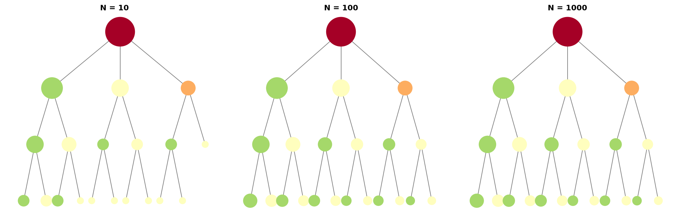
Figure 10.1 shows the morphological evolution of the MCTS search tree under different simulation counts. The three subplots, from left to right, correspond to N=10, 100, and 1000 simulations respectively:

Left (N=10): The tree is nearly symmetrical, with similar visit counts (similar node sizes) for each branch. At this stage, exploration is insufficient; UCB has not yet distinguished good from bad paths.
Middle (N=100): Asymmetry begins to emerge. Good branches (green nodes, high win rate) are prioritized for exploration, and nodes become noticeably larger. Bad branches (red nodes) have reduced visit counts.
Right (N=1000): Highly asymmetric. The optimal path is repeatedly visited (largest green node), suboptimal paths are moderately explored, and bad paths are nearly abandoned (small red nodes).

Key observation: Node size is proportional to visit count, and color represents average win rate (green = high, red = low). This asymmetric growth is precisely the core of the UCB algorithm — concentrating limited simulation budget on the most promising paths.

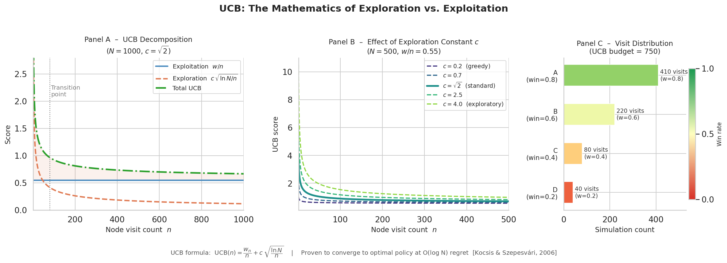
Figure 10.2: The exploration-exploitation tradeoff of UCB

Figure 10.2 shows how the exploration term and exploitation term in the UCB formula change with node visit count:

UCB (n) = \underset{exploitation term}{\underset{⏟}{average win rate}} + c \cdot \underset{exploration term}{\underset{⏟}{\sqrt{\frac{\ln N}{n}}}}

Blue curve (exploitation term): Average win rate converges to the true value (~0.7) as visit count increases. Early fluctuations are large; it stabilizes later.
Red curve (exploration term): $\sqrt{\ln N / n}$ decays with visit count. As visits increase, the exploration bonus decreases.
Green dashed line (total UCB): Sum of the two terms. Early on, the exploration term dominates (red is high); later, the exploitation term dominates (blue is stable).

The transition point is at n≈30: At this point, the contributions of the exploration and exploitation terms are roughly equal. Before this, it is "bold exploration"; after, "precise exploitation." This balance point is controlled by the constant $c$ — the larger $c$ is, the more aggressive the exploration.

VIII. Thought Experiment: When Search Becomes Gradient Descent

MCTS is nearly perfect on Tic-Tac-Toe because it exhausts the possibilities. But exhaustion is expensive — each move requires hundreds of simulations. If the state space has a continuous structure, why climb a discrete tree?

Let us do a thought experiment: encode board states as embedding vectors, encode board rules as a causal graph, and turn search into gradient descent in the embedding space.

This is what the CocDo project does — a causal world model that fuses Pearl's do-calculus with COC type theory.

8.1 The Causal World Operator: do() as β-reduction

The core of CocDo is a neural structural causal model: each variable (the 9 cells of Tic-Tac-Toe) is a D-dimensional embedding vector, and causal edges connect cells that share winning lines.

python

# Pseudocode: the core of the causal world operator
class NeuralSCM:
    def __init__(self, var_names, A, E, U):
        self.var_names = var_names  # ["c0", "c1", ..., "c8"]
        self.A = A                  # (9,9) causal weight matrix
        self.E = E                  # (9, D) embedding vectors
        self.U = U                  # (9, D) exogenous noise
    
    def do(self, var, value):
        # Pearl's do-calculus: cut incoming edges
        A_do = self.A.copy()
        idx = self.var_names.index(var)
        A_do[:, idx] = 0  # cut all edges pointing to var
        return NeuralSCM(self.var_names, A_do, self.E, self.U)
    
    def step(self, interventions):
        # One step of causal propagation: E_next = A_do^T @ E_do + U
        E_cur = self.E.copy()
        for var, val in interventions.items():
            idx = self.var_names.index(var)
            E_cur[idx] = val * E_cur[idx] / np.linalg.norm(E_cur[idx])
        
        A_do = self.A.copy()
        for var in interventions:
            idx = self.var_names.index(var)
            A_do[:, idx] = 0
        
        E_next = A_do.T @ E_cur + self.U
        return E_next

Key insight: do() is not a matrix operation, but a β-reduction in λ-calculus. In COC type theory, each edge X → Y is encoded as a dependent Π-type Π(X: Typeᵢ). Typeⱼ, where i < j ensures acyclicity. do(X=v) is subst(mechanism, X, Const(v)) then β-reduction.

8.2 Gradient Planning vs. Tree Search

Now let's look at two solutions for Tic-Tac-Toe:

MCTS (Tree Search):

python

def mcts_move(board, player, n_rollouts=500):
    # Build search tree, UCB1 selection, random simulation, backpropagation statistics
    # Time complexity: O(rollouts × depth)
    return best_move

CausalPlanner (Gradient Planning):

python

def planner_move(board, scm, player):
    # Encode board state as embeddings
    E_cur = board_to_embedding(board, scm.E, player)
    
    # Define targets: maximize embedding norms on winning lines
    target = {"c4": 1.8, "c0": 1.5, ...}  # center > corner > edge
    
    # Gradient descent to optimize intervention energy
    planner = CausalPlanner(scm)
    result = planner.plan(
        E_init=E_cur,
        target=target,
        interv_nodes=empty_cells(board),
        lr=0.1,
        steps=80
    )
    # Time complexity: O(steps × N × D)
    return max(empty_cells, key=lambda c: result["a_opt"][c])

Energy function: E(a) = Σⱼ (‖E_next[j]‖ - target_j)². Gradient descent finds intervention values that make embedding norms approach the targets.

8.3 Experimental Results: First Player Wins All; Second Player Partially Fails

Running python examples/demo_tictactoe.py --games 50:

Matchup A: Planner(X) vs MCTS(O)  — Planner moves first
  50/50  Planner=50  Draw=0  MCTS=0

Matchup B: MCTS(X) vs Planner(O)  — MCTS moves first  
  50/50  Planner=7   Draw=31  MCTS=12

Interpretation:

When moving first, gradient planning wins all: starting from an empty board, the gradient signal is clear — the center embedding norm is maximal, corresponding to the optimal first move.
When moving second, partial failures: when the board is complex (requiring multi-step lookahead), the gradient may get trapped in local optima, missing forced blocks.

This is not a bug; it is a feature: gradient planning captures continuous heuristics — "how good does this position look," rather than "search all possible outcomes." It replaces win-rate statistics in tree search with geometric distances in the embedding space.

8.4 Hands-On: Run the Tic-Tac-Toe Match

bash

git clone https://github.com/lizixi-0x2f/CocDo.git
cd CocDo
python examples/demo_tictactoe.py --games 20 --rollouts 200

Observe:

Gradient planning performs perfectly in simple positions (opening, direct wins/blocks)
It may make mistakes in complex positions (requiring 2+ move lookahead)
Computation speed comparison: gradient planning O(80×9×16) ≈ 11,520 floating-point operations vs MCTS O(200×depth) state evaluations

Discussion questions:

Under what circumstances does the gradient signal mislead? (When the optimal path requires temporarily "getting worse")
What game knowledge does the causal graph encode? (The topology of winning lines)
What future direction for AI planning does this suggest? (Continuous representation + gradient optimization vs discrete search)

MCTS is discrete exhaustive search; CausalPlanner is continuous heuristics. This is not a question of which is better, but rather two ontologies of search: one climbs a state tree, one flows through an embedding space. Gradient descent is not "approximate tree search"; it is something entirely different — replacing win rates in the tree with distances in the vector space. Acknowledging this difference is more important than pretending they are in competition.

X. Search for Large Language Models: From Chain-of-Thought to Reinforcement Learning

After 2022, the search problem gained a new dimension: a language model itself is a state space. Each reasoning step is no longer a stone placed on a board, but a piece of text — mathematical derivation, logical analysis, a line of code.

This gives rise to a profound question: how can we make LLMs perform effective search in the language reasoning space?

MCTS's answer is: build a tree, simulate, backpropagate. But for language models, "one simulation" means running the entire forward pass, with extremely high computational cost. Moreover, the language reasoning space is continuous, and the branching factor is infinite — you cannot exhaust all possibilities for "the next sentence."

Two different technical routes give two starkly different answers.

10.1 GPT-o1: Process Reward Models and Policy Distillation

In September 2024, OpenAI released the o1 model series. Its core innovation lies not in model architecture, but in search strategy.

o1's technical route can be summarized as a three-layer architecture:

Layer 1: Process Reward Model (PRM)

Traditional reinforcement learning rewards are given at the endpoint — correct answer +1, wrong answer -1. But in reasoning tasks, this is too sparse: a math problem requiring 20 derivation steps only gets judged right or wrong at step 20.

The PRM idea is: score every intermediate step. Given the k-th step in a reasoning chain, the PRM outputs the probability that this step is "going in the right direction":

r_{k} = PRM (s_{0}, a_{1}, a_{2}, \dots, a_{k})

This is equivalent to converting sparse terminal rewards into dense process rewards, allowing search to receive feedback at every step.

Layer 2: Policy Model Guidance in Tree Search

With the PRM in place, o1 uses a policy model (a fine-tuned language model) to perform MCTS-like search in the reasoning step space:

Selection: use the policy model to generate $K$ candidate reasoning steps
Evaluation: PRM scores each candidate step
Expansion: select the highest-scoring step to continue expansion
Backpropagation: use the final result to update the PRM and policy model in reverse

This is the first time tree search and language model reasoning have been systematically combined. The Chain of Thought (CoT) is no longer a single linear derivation, but a search tree growing in the reasoning space.

Layer 3: Knowledge Distillation Compresses Search

Search is great, but slow. What o1 actually runs during inference is a distilled policy model — during training, it has seen a large number of high-quality reasoning trajectories generated by tree search, and has learned to "internally" simulate the search process, without needing to explicitly build a tree during inference.

This is analogous to human chess players: a novice needs to calculate all variations; an expert knows the best move at a glance — because the expert has "internalized" search into intuition.

This is a historic moment for Chain of Thought: CoT is no longer just a technique that improves accuracy; it has become the infrastructure for language models to perform systematic search in the reasoning space.

10.2 DeepSeek-R1: Ditch the PRM, Group-Competitive Reinforcement Learning

In early 2025, DeepSeek released the R1 model, with a technical route that forms a stark contrast to o1: completely no PRM.

o1's route has a fundamental bottleneck: how is the PRM trained?

To train a PRM, you need humans to annotate every intermediate reasoning step as "right/wrong." This is an extraordinarily expensive data engineering effort — a problem requiring 20 derivation steps needs annotation at every step, making data costs 20 times that of terminal annotation.

And a deeper problem is: who judges whether an intermediate step is right? Some reasoning paths that look "wrong" ultimately yield the correct answer; some paths that look "right" fail at the last step. The correctness of intermediate steps depends on the outcome, but the PRM needs to score without knowing the outcome. This is an essential difficulty.

DeepSeek-R1's solution is Group Relative Policy Optimization (GRPO):

Core idea: no absolute scoring needed, only relative ranking

For the same problem, let the model generate $G$ complete reasoning trajectories (answer chains):

{o_{1}, o_{2}, \dots, o_{G}} \sim π_{θ} (\cdot ∣ q)

Judge right/wrong only at the endpoint: $r_{i} = 1$ if the i-th trajectory yields the correct answer, otherwise $r_{i} = 0$ .

Then compute within-group relative advantage — which trajectories are better than the group average?

A_{i} = r_{i} - \frac{1}{G} \sum_{j = 1}^{G} r_{j}

Use this relative advantage to update the policy:

L_{GRPO} = - E [\frac{π_{θ} (o_{i} ∣ q)}{π_{θ_{old}} (o_{i} ∣ q)} \cdot A_{i}]

The profundity of this design:

No PRM needed: reward signals come only from terminal right/wrong judgments, completely eliminating the need for intermediate step annotation
Within-group competition: trajectories in the same group form a competitive relationship — those "better than the average" receive positive gradients, those "worse than the average" receive negative gradients
Emergent search: the model spontaneously learns "self-verification" during training — generating multiple reasoning paths, internally comparing them, and keeping the better one

This is a profound innovation in reinforcement learning: replacing explicit process supervision (PRM) with implicit within-group competitive pressure.

10.3 A Philosophical Comparison of the Two Routes

Dimension	GPT-o1 Route	DeepSeek-R1 Route
Process supervision	Explicit PRM, step-by-step scoring	No PRM, terminal reward only
Search method	Explicit tree search + distillation	GRPO within-group competition
Data requirement	High (process annotation)	Low (answer annotation only)
Computational cost	Low training, high inference	High training, low inference
Emergent ability	Transmitted via distillation	Spontaneously emerges via competition

From the MCTS perspective, the two routes correspond to two different search strategies:

The o1 route is more like supervised tree search: PRM is a hand-designed heuristic function, and the policy model is a prior guided by human data. It is highly dependent on human knowledge, but performs powerfully in domains with data.

The DeepSeek-R1 route is more like unsupervised random search + selection pressure: GRPO is equivalent to letting $G$ random walk trajectories compete on the same problem, with natural selection keeping the good paths. It does not depend on human judgment of "process," but needs a large number of samples to generate sufficient competitive pressure.

This is a profound tension: the more precise the process supervision, the more it depends on human knowledge; the less it depends on human knowledge, the more it needs spontaneous competitive emergence.

Chain of Thought exposes this tension in the era of language models. In the Go era, the answer to this tension was AlphaGo Zero — completely abandoning human game records, relying on the competitive selection of self-play. In the language reasoning era, this tension has no final answer yet.

XI. The Philosophy of Search: Computation as Reasoning

MCTS reveals a profound fact: reasoning does not require "understanding," only effective search.

AlphaGo does not know the aesthetics of Go, does not understand concepts like "thickness" or "territory." It only knows: in this state, which action's simulated win rate is highest.

But this is enough. Through millions of simulations, MCTS found moves that humans had not discovered in thousands of years.

This raises a philosophical question: if search is powerful enough, do we still need "understanding"?

One view holds: understanding is a shortcut for search. Human players, by understanding Go principles, can quickly prune, without needing to search all possibilities. But if computational resources are infinite, search can replace understanding.

Another view holds: understanding is the foundation of generalization. MCTS is strong at Go, but switching to a different game requires retraining. Humans understand abstract concepts like "strategy" and "trade-off" and can quickly transfer to new games.

ADS's entropy regularization offers a third perspective: search can be reshaped in real-time through dynamic constraints. There is no need to "solidify search as weights"; instead, use entropy barriers to repel high-uncertainty states at each step of reasoning.

This is analogous to potential fields in physics: rather than pre-computing all paths, you feel the potential energy gradient at each position and naturally move in the direction of lower potential energy.

Search is powerful, but expensive. In the next chapter, we will confront the economics of reasoning: how to produce equally good reasoning with less computation?

Unresolved

What is the generalization boundary of entropy regularization? ADS is effective on arithmetic tasks, but on tasks requiring multi-layer abstraction, small models exhibit "confident hallucination." What is the relationship between the entropy barrier and model capacity?
Can topological reshaping be generalized to other reasoning tasks? Logarithmic barriers work in LLM reasoning, but what about symbolic reasoning, theorem proving, and other discrete search spaces?
What is the optimal balance of exploration and exploitation? How is the constant c in the UCB formula chosen? Do different problems require different c?
Can MCTS be generalized to continuous action spaces? The actions in Go and Tic-Tac-Toe are discrete. How can MCTS be applied to continuous-action problems like robot control and continuous optimization?
Where is the boundary between search and reasoning? Theorem proving can be viewed as search, but can a mathematician's "insight" be captured by search?
Is there an inherent difficulty in intermediate step annotation for PRM? If a reasoning path that "looks wrong" ultimately yields the correct answer, is that step right or wrong? Does this annotation difficulty mean that PRM can never provide truly reliable process supervision?
Where does GRPO's within-group competitive pressure come from? If all $G$ trajectories answer correctly (or all incorrectly), $A_{i} = 0$ , the gradient vanishes, and the model cannot learn. This means GRPO requires precise calibration of task difficulty — not too hard (all wrong), not too easy (all correct). Is this calibration a solvable engineering problem, or a fundamental limitation?

Chapter 10: The Art of Search: Navigating the Reasoning Space ​

I. Move 37, March 2016 ​

II. The Curse of Search Space ​

III. MCTS: The Wisdom of Random Sampling ​

IV. The UCB Formula: The Mathematics of Exploration and Exploitation ​

V. Hands-On: Playing Tic-Tac-Toe with MCTS ​

VI. From Search to Intuition: Entropy Regularization in ADS ​

VII. Pseudocode: MCTS, ADS, and Causal Planning ​

IX. Visualization: The Asymmetric Growth of the Search Tree ​

VIII. Thought Experiment: When Search Becomes Gradient Descent ​

8.1 The Causal World Operator: do() as β-reduction ​

8.2 Gradient Planning vs. Tree Search ​

8.3 Experimental Results: First Player Wins All; Second Player Partially Fails ​

8.4 Hands-On: Run the Tic-Tac-Toe Match ​

X. Search for Large Language Models: From Chain-of-Thought to Reinforcement Learning ​

10.1 GPT-o1: Process Reward Models and Policy Distillation ​

10.2 DeepSeek-R1: Ditch the PRM, Group-Competitive Reinforcement Learning ​

10.3 A Philosophical Comparison of the Two Routes ​

XI. The Philosophy of Search: Computation as Reasoning ​

Unresolved ​

Further Reading ​

Chapter 10: The Art of Search: Navigating the Reasoning Space

I. Move 37, March 2016

II. The Curse of Search Space

III. MCTS: The Wisdom of Random Sampling

IV. The UCB Formula: The Mathematics of Exploration and Exploitation

V. Hands-On: Playing Tic-Tac-Toe with MCTS

VI. From Search to Intuition: Entropy Regularization in ADS

VII. Pseudocode: MCTS, ADS, and Causal Planning

IX. Visualization: The Asymmetric Growth of the Search Tree

VIII. Thought Experiment: When Search Becomes Gradient Descent

8.1 The Causal World Operator: do() as β-reduction

8.2 Gradient Planning vs. Tree Search

8.3 Experimental Results: First Player Wins All; Second Player Partially Fails

8.4 Hands-On: Run the Tic-Tac-Toe Match

X. Search for Large Language Models: From Chain-of-Thought to Reinforcement Learning

10.1 GPT-o1: Process Reward Models and Policy Distillation

10.2 DeepSeek-R1: Ditch the PRM, Group-Competitive Reinforcement Learning

10.3 A Philosophical Comparison of the Two Routes

XI. The Philosophy of Search: Computation as Reasoning

Unresolved

Further Reading