Chapter 5: The Trap of Fitting — Statistical Correlation Is Not Reasoning
After a model has seen a million cats, does it know what a cat is?
I. A Disturbing Experiment
In 2021, Bender et al. published a paper with a blunt title: On the Dangers of Stochastic Parrots.
The title is not a metaphor; it's a diagnosis.
The paper's core argument: large language models, no matter how much text they are trained on, are essentially doing statistical pattern matching — they have learned which word sequences frequently co-occur in the training corpus, and then reproduce these patterns during generation. Like a parrot that, after hearing enough conversations, can say "hello" or "goodbye" at the right moment, but doesn't understand the meaning of these words.
This analogy stings, because it touches a deeper question: between statistical correlation and causal understanding, there is a chasm.
Let me show you a more concrete example.
In 2023, Hodel and West ran a simple test. They gave GPT-3 letter-string analogical reasoning tasks — the same tasks on which Webb et al. had claimed in 2023 that GPT-3 had "emerged" analogical reasoning abilities.
The original task went like this:
Input: abc -> abd, kji -> ?
Expected output: kjj
This is a simple rule of "shift the last letter forward by one." GPT-3 performs well on this task.
Then Hodel and West made the simplest variation: change the letter-string length from 3 to 4, or slightly shuffle the order of the alphabet.
GPT-3's performance immediately collapsed.
Not "dropped slightly" — collapsed. Accuracy went from near 100% to near random guessing. Yet human performance on these variants barely changed, because humans understand the rule itself, not the surface pattern on a specific length and a specific alphabet.
This is the core question of this chapter: When a model learns by minimizing training error, what does it learn?
II. The Compact of Empirical Risk Minimization
Let's make this question mathematically clear.
The standard paradigm of supervised learning is Empirical Risk Minimization (ERM). Given training data
Here
Empirical Risk Minimization (ERM): What Is Model Training Doing?
Empirical Risk Minimization is the underlying logic of most machine learning training. In plain terms: make the model's prediction error on the training data as small as possible.
A few key terms:
- Hypothesis
: The model itself (e.g., a neural network), which given input , outputs prediction - Loss function
: A function that quantifies "how bad the prediction is" — e.g., predicting "cat" when the label is "dog" yields a high loss; predicting correctly yields a low loss - Empirical risk
: The average loss across all training samples — minimizing this means "getting the model to answer as correctly as possible on the training set"
The core problem: Minimizing training error ≠ truly understanding the pattern. The model may just have "memorized the answers" (overfitting), or learned surface patterns rather than underlying mechanisms. This is exactly what this chapter interrogates: what does ERM learn?
The theoretical guarantee of ERM comes from a simple intuition: if the training data is sampled i.i.d. from some distribution
How fast is this convergence? Statistical learning theory tells us that for finite hypothesis spaces, the convergence rate is
But here is an overlooked premise: are the objective optimized by ERM and the objective we truly care about the same thing?
Let me unpack this question.
What is ERM doing? It is searching for a function
But what does "reasoning" require? Reasoning requires the model to capture the causal mechanism between
These two are not the same thing.
The classic results of statistical learning theory — for example, the framework established by Vapnik and Chervonenkis in the 1970s — concern generalization bounds:
This inequality tells us: if the hypothesis space is not too complex, a model with low training error will also have low test error.
But note the assumption here: test data and training data come from the same distribution
This assumption almost never holds in reality.
Training data is the data you could collect — perhaps from specific hospitals, specific time periods, specific populations. Test data is the data the model encounters after deployment — perhaps from different hospitals, different seasons, different populations.
Distribution Shift is the norm, not the exception.
And when distribution shift occurs, the "correlations that are effective on the training data" that ERM learned can completely fail.
A Pause
The model memorized the training set — we call that overfitting, it's a mistake, we penalize it.
But what if the model memorized the entire internet?
What do we call that?
GPT-4's training data scale is approximately a large sample of all the text ever written by humanity. If it "memorized" all of that, what is the essential difference from overfitting? — Is it scale, or something else?
One more question: when distribution shift occurs, ERM fails. But humans, when facing distribution shift, also sometimes fail — we misjudge in unfamiliar cultures, make naive mistakes in new domains.
Then, are the flaws of ERM unique to machine learning, or are they shared by all inductive learning systems? Including yourself?
Set this question aside for now.
III. Shortcut Learning: When Correlation Is Easier Than Causation
Here's a thought experiment.
Suppose you want to train a model to recognize "cows." The training set has 1000 cow photos, of which 950 have grassland backgrounds, and 50 have beach backgrounds (some seaside farm).
What will ERM learn?
If the model is simple enough, it might learn: "If the background is grassland, predict cow." This rule achieves 95% accuracy on the training set — very good.
But does this rule capture the essence of "cow"? Obviously not. When you deploy this model at a beach farm, it will misclassify every cow.
This is Shortcut Learning — the model learns to exploit spurious correlations in the training data, rather than genuine causal features.
In their 2020 review, Geirhos et al. systematically summarized this phenomenon. They pointed out that shortcut learning is ubiquitous in deep learning:
Texture bias: ImageNet-trained models rely more on texture than shape for classification, while humans do the opposite
Background dependency: Object detection models exploit background statistics (e.g., "boats usually appear on water") as shortcuts
Dataset bias: Sentiment analysis models over-rely on certain high-frequency words (like "terrible," "amazing") while ignoring the overall semantics of the sentence
Why does this happen?
Because ERM has no mechanism to distinguish "useful correlations" from "spurious correlations." As long as some feature correlates with the label in the training data, ERM will exploit it — regardless of whether that correlation still holds outside the training distribution.
In 2022, Puli et al.'s research revealed a deeper reason: even when spurious features (shortcuts) provide no additional information — that is, when stable features already fully determine the label — default ERM (gradient descent + cross-entropy) still preferentially relies on shortcuts.
Why? Because gradient descent implicitly maximizes the classification margin. And in the linearly separable case, the max-margin solution tends to be the one that exploits both stable features and shortcuts, even though stable features alone would achieve zero training error.
This is not overfitting — the training error is already zero. This is a problem of inductive bias: the combination of gradient descent + cross-entropy naturally prefers a certain type of solution, and this solution, when shortcuts exist, over-relies on shortcuts.
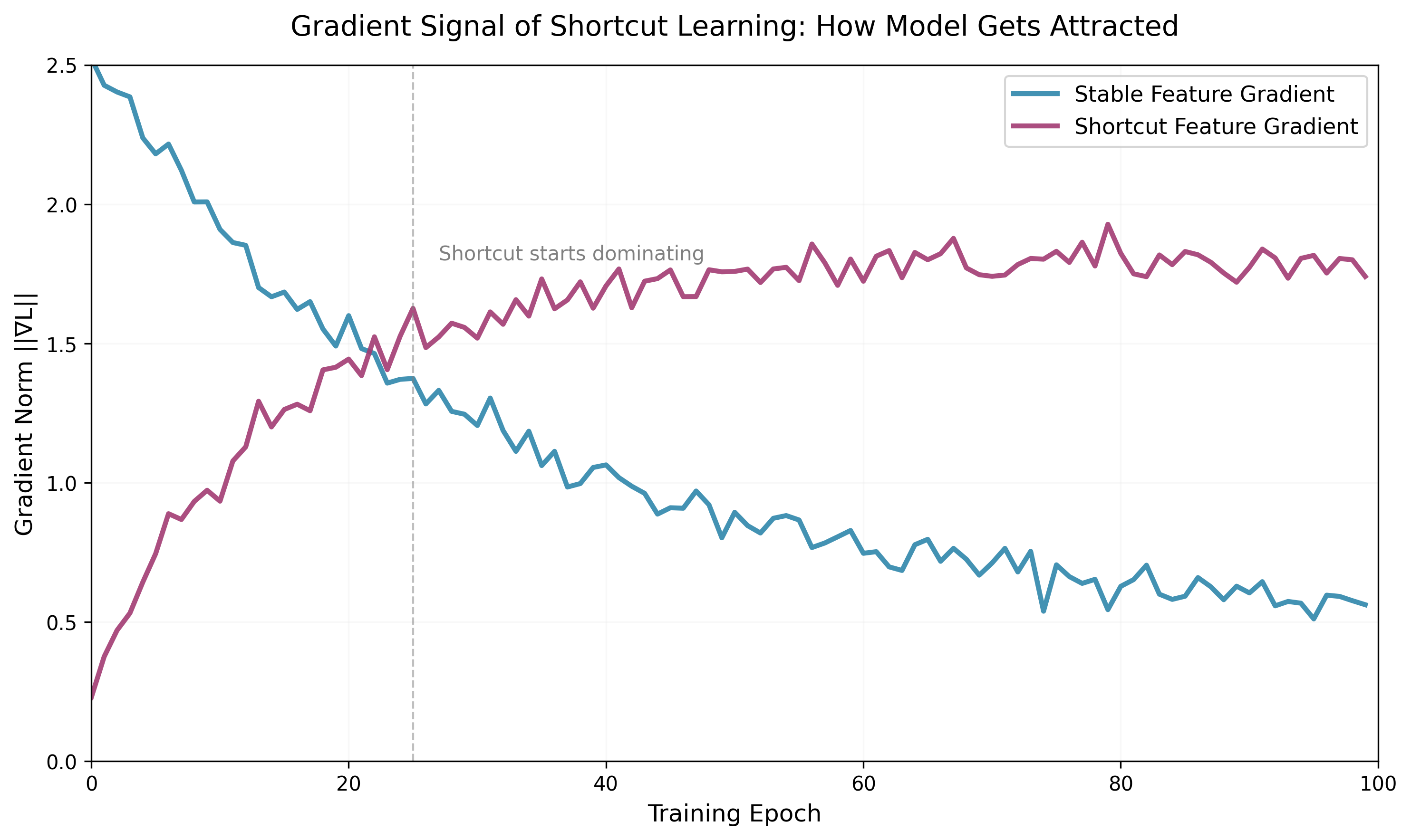
Figure 1: During training, the gradient norm of shortcut features grows rapidly and stays high, while the gradient of stable features gradually decays. This indicates that the model is progressively attracted to shortcuts during optimization, even though stable features alone suffice for the task.
Let me use a more formalized framework to illustrate this.
IV. The Causal Graph Perspective: Stable Features vs. Spurious Features
Suppose the data-generating process can be described by a causal graph. There are three variables:
: the label (e.g., "whether it is a cow") : stable features (e.g., the cow's shape, texture) : shortcut features (e.g., whether the background is grassland)
The true causal relationships are:
That is, the label
But this correlation is not causal.
What does ERM see? ERM sees the joint distribution
If
The problem is: when test data comes from a different distribution, where the correlation between
This is not the model being "not smart enough." This is a structural limitation of ERM: ERM optimizes
Pearl's causal ladder tells us that to answer interventional questions ("If I change the background to beach, can the model still recognize cows?"), what you need is not conditional probabilities but a causal model.
But ERM can only access observational data; it cannot distinguish correlation from causation.
V. The Stochastic Parrot Hypothesis: Repeating Is Not Understanding
Now let's return to the question from the beginning of this chapter: Are large language models stochastic parrots?
The core of this question is not whether models are "conscious" or "understanding" — those are philosophical questions that we set aside for now. The core is: to what extent can a model's behavior be explained by "memorization + retrieval of patterns in the training data"?
In 2025, Zhao et al.'s research proposed a key test: Is Chain-of-Thought (CoT) reasoning genuine reasoning, or a mirror of the training data distribution?
Their experimental design was ingenious. They constructed a fully controllable environment, DataAlchemy, trained language models from scratch, and then systematically varied the distributional differences between training data and test data:
Task distribution shift: during training, models saw addition; during testing, they did multiplication
Length distribution shift: during training, models saw 3-digit arithmetic; during testing, they did 5-digit arithmetic
Format distribution shift: during training, models saw the "step 1, step 2" format; during testing, they got "first, second"
The results were devastating: CoT reasoning significantly degrades under all three types of distribution shift. The model is not "reasoning" — it is "pattern matching." It has learned, in the training data, what kind of input corresponds to what kind of reasoning chain format, and then reproduces that format during testing.
When the distribution of test data differs from that of training data, this reproduction fails.
This is the same phenomenon as GPT-3's collapse on letter-string analogy in Section I: the model learns surface statistical regularities, not underlying abstract rules.
But here is a deeper question.
Bender et al.'s "stochastic parrot" critique implicitly assumes: if a model is only doing statistical pattern matching, then its capabilities have an upper bound — it cannot transcend the statistical structure of the training data.
But is this assumption correct?
In 2023, Wei et al. proposed a counterargument: even if models are only doing pattern matching, if the training data is large enough and diverse enough, pattern matching itself may suffice to produce behaviors that look like "reasoning."
This is a debate about emergence: when model scale and data scale grow to some critical point, does a qualitative change occur?
The current evidence is mixed.
On one hand, we have indeed seen some surprising capabilities — for example, GPT-4's performance on certain reasoning tasks has approached the human average.
On the other hand, the fragility of these capabilities under distribution shift suggests they may still be "complex pattern matching," not genuine abstract reasoning.
The key test is: can the model produce correct behavior on novel combinations that never appeared in the training data?
This is what the next section addresses: distribution shift as a touchstone.
VI. Distribution Shift: The Touchstone of Reasoning Ability
If a model truly "understands" what it is doing, then when the distribution of input data changes, its performance should degrade gracefully — not collapse.
This is a hypothesis that can be precisely tested.
In-Distribution (ID) performance measures how well the model performs on data similar to the training data. This is standard test-set evaluation.
Out-of-Distribution (OOD) performance measures how well the model performs on data outside the training distribution. This is true generalization ability.
Let me show you several concrete examples of how distribution shift exposes model fragility.
Example 1: Shortcuts in Medical Image Segmentation
In 2024, Woodland et al. studied the OOD detection of deep learning models on medical image segmentation tasks. They found: models trained on liver segmentation tasks, when encountering images from different hospitals and different scanners, experience significant performance drops.
The problem was not image quality — the new images were of good quality. The problem was that the model learned device-specific artifacts in the training data as shortcuts.
For example, a specific CT scanner model produces a particular noise pattern at a certain position in the image. The model learned to exploit this noise pattern to assist segmentation — because in the training data, this noise pattern was highly correlated with the location of the liver.
But when switching to a different scanner model, this noise pattern disappears, and the model's segmentation accuracy collapses.
Example 2: Spurious Correlations in Natural Language Understanding
In 2023, Shuieh et al. systematically evaluated the robustness of three post-training algorithms (SFT, DPO, KTO) under spurious correlations.
They constructed three types of tasks — mathematical reasoning, instruction following, document Q&A — and introduced varying degrees of spurious correlations (10% vs. 90%) into the data.
The results showed: all models significantly degrade under high spurious correlation. Preference learning methods (DPO/KTO) were relatively robust on mathematical reasoning tasks, but on complex, context-intensive tasks, supervised fine-tuning (SFT) was actually stronger.
What does this indicate? It indicates that no single training method universally resists shortcut learning. The optimal strategy depends on the task type and the nature of the spurious correlation.
Example 3: Distributional Fragility of CoT Reasoning
Returning to Zhao et al.'s DataAlchemy experiment. Their core finding: CoT reasoning is a fragile mirror of the training data distribution.
When any one of the three dimensions — task, length, format — shifts, the effectiveness of CoT drops significantly. This indicates that what the model has learned is not "how to reason," but "what a reasoning chain looks like in the training data."
Worse, the model's failure mode under distribution shift is systematic, not random. It doesn't make occasional mistakes; it consistently fails on specific types of inputs — because those inputs trigger patterns that don't exist in the training data.
These three examples point to the same conclusion: distribution shift is not an edge case; it is the core test. If a model only performs well in-distribution, then what it has learned is likely statistical correlation, not causal mechanism.
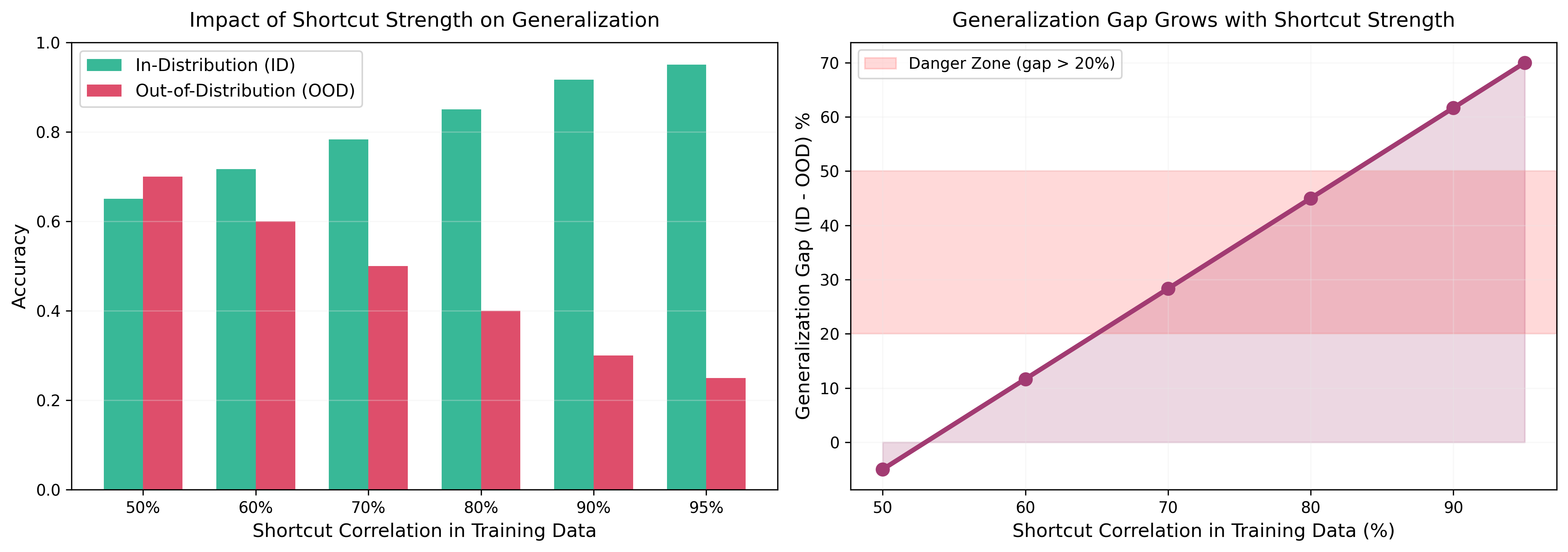
Figure 2: Left panel shows that as the shortcut correlation in training data increases, ID accuracy improves but OOD accuracy declines. Right panel shows that the generalization gap (ID - OOD) grows linearly with shortcut strength; when shortcut correlation exceeds 80%, the generalization gap enters the danger zone (>20%). This quantifies the destructive impact of shortcut learning on out-of-distribution generalization.
VII. Why ERM's Inductive Bias Is Not Enough
Now we arrive at the most critical point of this chapter.
The problem is not ERM itself — ERM is a reasonable learning principle. The problem is: ERM, combined with standard optimization algorithms (gradient descent) and loss functions (cross-entropy), produces an inductive bias that is unsuitable for learning causal structures.
Let me unpack this argument.
Inductive Bias is the implicit assumption of a learning algorithm — it determines which hypothesis, among the many that can fit the training data, the algorithm will choose.
What is the inductive bias of gradient descent + cross-entropy?
In the linearly separable case, gradient descent converges to the max-margin solution — the solution that maximizes the distance from the classification boundary to the nearest training sample.
In many situations, this is good. A larger margin usually means better generalization — because it is more robust to small perturbations of the training data.
But when shortcuts are present, the max-margin solution tends to be the one that simultaneously exploits stable features and shortcuts.
Why? Because if you use two features simultaneously, you can push the classification boundary farther — even if one of those features (the shortcut) will fail out-of-distribution.
Puli et al.'s 2023 research precisely characterized this phenomenon. They proved: in a simple linear perception task, even when stable features already fully determine the label, gradient descent will still assign non-zero weight to shortcuts — because that maximizes the margin.
What is the solution?
One direction is to change the inductive bias. For example, instead of pursuing max-margin, pursue uniform margin — making the distance from all training samples to the classification boundary as equal as possible.
Puli et al.'s MARG-CTRL (Margin Control) follows this approach. By adjusting the loss function, it encourages the model to produce a uniform-margin solution, thereby reducing dependency on shortcuts.
Another direction is to explicitly model causal structure. This requires going beyond purely observational data, introducing interventions or counterfactual reasoning — this is the topic of Chapter 6.
But even without introducing causal reasoning, we can mitigate shortcut learning through smarter training strategies.
VIII. Mitigation Strategies: From Data Augmentation to Adversarial Training
If we know where the shortcuts are, what can we do?
Strategy 1: Data Augmentation
The most direct approach is to increase the diversity of training data and break spurious correlations.
For example, in the cow recognition case, if you can collect enough "cow on beach" images, the model won't over-rely on the "grassland background" shortcut.
But this approach has two problems:
First, you need to know what the shortcut is. In real-world scenarios, shortcuts are often hidden — you don't know what spurious correlation the model is exploiting.
Second, even if you know the shortcut, collecting sufficiently diverse data can be extremely expensive or infeasible.
Strategy 2: Reweighting Training Samples
If certain training samples are "too easy" — the model can predict correctly using shortcuts — then reduce the weight of those samples, forcing the model to learn from harder samples.
This is the idea behind Li et al.'s 2020 Tilted ERM. By introducing a "tilt" parameter
When
By adjusting
Strategy 3: Adversarial Training
Another approach is to explicitly generate "adversarial examples" — samples on which the model would fail by relying on shortcuts — and then train on those samples.
In 2018, Sricharan and Srivastava proposed: use GANs to generate samples on which the model has high confidence but which are actually OOD, and then maximize the model's entropy (uncertainty) on those samples.
This forces the model not to be overconfident on out-of-distribution inputs, thereby reducing dependency on shortcuts.
Strategy 4: Causal Regularization
If we have prior knowledge about the causal structure, we can encode it into a regularization term.
For example, if we know that some feature
Here
But all these methods share a common limitation: they require some form of supervisory signal — either prior knowledge about shortcuts, or OOD data, or manually labeled hard examples.
In the completely unsupervised setting, detecting and mitigating shortcut learning remains an open problem.
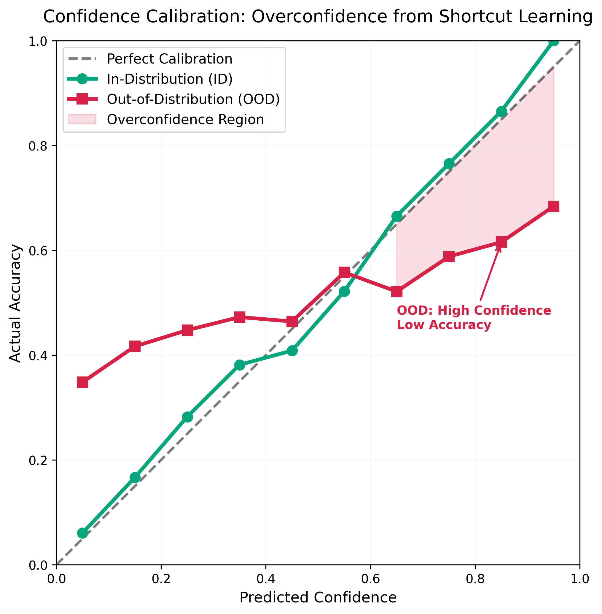
Figure 3: The confidence calibration curve reveals the most dangerous consequence of shortcut learning — overconfidence. ID data (green) is well-calibrated along the diagonal, while OOD data (red) deviates severely: the model's actual accuracy at high confidence (0.8-0.9) is only 0.6-0.7. The shaded region indicates the overconfidence zone, where the model confidently gives wrong predictions without any uncertainty warning.
IX. Pseudocode: Shortcut Detection and OOD Generalization Test
Let me formalize the core algorithms discussed above.
Algorithm 1: Gradient-Based Shortcut Detection
import torch

def shortcut_detection(model, dataloader, shortcut_indices, stable_indices, tau=0.5):
    """
    Gradient-based shortcut detection.
    shortcut_indices: list of column indices of shortcut features in the input
    stable_indices:   list of column indices of stable features in the input
    Returns: shortcut dependency score S (higher means more reliance on shortcuts)
    """
    model.eval()
    ratios = []
    criterion = torch.nn.CrossEntropyLoss()

    for x, y in dataloader:
        x = x.requires_grad_(True)
        output = model(x)
        loss = criterion(output, y)
        loss.backward()

        g = x.grad  # shape: (batch, n_features)
        g_c = g[:, shortcut_indices].norm(dim=1)   # Norm of gradients w.r.t. shortcut features
        g_s = g[:, stable_indices].norm(dim=1)     # Norm of gradients w.r.t. stable features
        ratio = g_c / (g_s + 1e-8)
        ratios.append(ratio.detach())

    S = torch.cat(ratios).mean().item()
    if S > tau:
        print(f"S={S:.3f} > τ={tau}: Model significantly relies on shortcut features")
    else:
        print(f"S={S:.3f} ≤ τ={tau}: Model mainly relies on stable features")
    return S
The intuition of this algorithm is: if the model over-relies on shortcuts, the gradient of the loss with respect to the shortcut features will be large — because changing the shortcut features significantly affects predictions.
Algorithm 2: Generalization Test Under Distribution Shift
def generalization_test(model, id_loader, ood_loader, device="cpu"):
    """
    Evaluate the model on ID and OOD test sets, report the generalization gap.
    """
    def evaluate(loader):
        model.eval()
        correct, total, high_conf_wrong = 0, 0, 0
        with torch.no_grad():
            for x, y in loader:
                x, y = x.to(device), y.to(device)
                logits = model(x)
                probs = torch.softmax(logits, dim=1)
                pred = probs.argmax(dim=1)
                conf = probs.max(dim=1).values
                correct += (pred == y).sum().item()
                # High-confidence but wrong predictions (overconfidence detection)
                high_conf_wrong += ((conf > 0.8) & (pred != y)).sum().item()
                total += y.size(0)
        return correct / total, high_conf_wrong / total

    acc_id,  hcw_id  = evaluate(id_loader)
    acc_ood, hcw_ood = evaluate(ood_loader)
    gap = acc_id - acc_ood

    print(f"ID  accuracy: {acc_id:.1%}")
    print(f"OOD accuracy: {acc_ood:.1%}")
    print(f"Generalization gap:   {gap:.1%}")
    if gap < 0.05:
        print("-> Good generalization; model may have learned stable features")
    elif gap < 0.20:
        print("-> Moderate generalization; partial reliance on shortcuts")
    else:
        print("-> Poor generalization; model severely relies on shortcuts")
    if hcw_ood > 0.1:
        print(f"⚠ OOD high-confidence error rate {hcw_ood:.1%}, overconfidence present")
    return acc_id, acc_ood, gap
Algorithm 3: Tilted ERM Training
import torch
import torch.nn as nn

def tilted_erm_train(model, dataloader, t=5.0, lr=1e-3, epochs=50):
    """
    Tilted ERM training: give higher weight to hard samples, reducing shortcut reliance.
    t > 0: larger means more focus on high-loss samples; t = 0 degenerates to standard ERM.
    """
    optimizer = torch.optim.Adam(model.parameters(), lr=lr)
    criterion = nn.CrossEntropyLoss(reduction="none")

    for epoch in range(epochs):
        model.train()
        for x, y in dataloader:
            losses = criterion(model(x), y)          # Per-sample losses
            # Tilted loss: log-sum-exp softens the maximum
            tilted_loss = (1.0 / t) * torch.log(
                (1.0 / len(losses)) * torch.sum(torch.exp(t * losses))
            )
            optimizer.zero_grad()
            tilted_loss.backward()
            optimizer.step()

    return model
When
X. A Brief Pause
Let me sort out what this chapter has done.
Empirical Risk Minimization is the standard paradigm of supervised learning. Its theoretical guarantees rest on a key assumption: training data and test data come from the same distribution.
But this assumption almost never holds in reality. Distribution shift is the norm, not the exception.
When distribution shift occurs, the "correlations that are effective on the training data" that ERM learned can completely fail. This is not a bug; it is a structural feature of ERM: ERM optimizes statistical correlation, not causal mechanism.
Shortcut learning is the concrete manifestation of this problem: the model learns to exploit spurious correlations in the training data, rather than genuine causal features. Worse, even when spurious features provide no additional information, the inductive bias of gradient descent + cross-entropy still leads the model to rely on them — because that maximizes the classification margin.
The Stochastic Parrot Hypothesis points out: large language models may merely be doing complex statistical pattern matching, not genuine reasoning. Their fragility under distribution shift — for example, the collapse of CoT reasoning under task, length, and format shifts — supports this hypothesis.
Methods to mitigate shortcut learning include data augmentation, sample reweighting, adversarial training, and causal regularization. But all these methods require some form of supervisory signal. In the completely unsupervised setting, detecting and mitigating shortcut learning remains an open problem.
This leads to the core question of Chapter 6: if statistical correlation is insufficient, what do we need? The answer is causal reasoning — not just observing
Correlation is a shortcut, not reasoning. In the next chapter, we will confront the question head-on: What is causation? And why observational data can never tell you the answer.
Unresolved
Are the "emergent capabilities" of large language models genuine qualitative change, or quantitative change in complex pattern matching? As model scale continues to grow, will the answer to this question change?
In the completely unsupervised setting, does a universal method exist to detect shortcut learning? Or does detecting shortcuts inherently require prior knowledge about the task?
Under what conditions is ERM's inductive bias (max-margin) beneficial, and under what conditions is it harmful? Is there a unified framework to characterize this trade-off?
If we train a neural network on purely random data, what kind of "shortcut" will it learn? Can this thought experiment tell us something about the nature of shortcut learning?
Does human learning also exhibit shortcut learning? If so, how do humans overcome it? What insights does this offer for designing better machine learning algorithms?
Try It Yourself: Construct a Shortcut Trap, Then Watch the Model Fall Into It
The core proposition of this chapter: ERM will exploit any correlation in the training data, regardless of whether that correlation is causal. You will verify this firsthand — not by understanding it intellectually, but by watching it happen.
Step 1: Design Your Shortcut Dataset
Choose a simple binary classification task, then deliberately implant a shortcut in the data.
Option A: Image Classification (Recommended)
Task: distinguish between two types of simple shapes (e.g., circles vs. squares)
Shortcut design: - Training set: 90% of circles placed on the left half of the image, 90% of squares placed on the right half - Test set (ID): maintain the same positional bias - Test set (OOD): reverse the positions — circles on the right, squares on the left
Option B: Text Classification
Task: sentiment classification (positive vs. negative)
Shortcut design: - Training set: append "Recommended!" to 90% of positive reviews, "Not recommended" to 90% of negative reviews - Test set (ID): maintain the same markers - Test set (OOD): remove all markers, keep only the review body
Your first question (answer before generating data): What do you think the model will learn? Will it rely on position/markers (shortcuts), or shape/semantics (stable features)? Why?
Step 2: Train a Standard ERM Model
Use the simplest architecture: - Images: 2-3 layer convolutional network - Text: simple LSTM or Transformer
Training objective: minimize cross-entropy loss until training accuracy > 95%
Do not do any special handling — just standard gradient descent + cross-entropy.
Record: - Training curve (loss vs. epoch) - Final training accuracy
Step 3: Evaluate on Three Test Sets
import numpy as np
import torch
import torch.nn as nn
from sklearn.metrics import accuracy_score

# ── Helper function: evaluate model accuracy ────────────────────────────────────
def evaluate(model, dataloader, device='cpu'):
    """Return the model's accuracy (0~1) on a given dataset."""
    model.eval()
    all_preds, all_labels = [], []
    with torch.no_grad():
        for X_batch, y_batch in dataloader:
            X_batch = X_batch.to(device)
            logits = model(X_batch)
            preds = logits.argmax(dim=1).cpu().numpy()
            all_preds.extend(preds)
            all_labels.extend(y_batch.numpy())
    return accuracy_score(all_labels, all_preds)

# 1. ID test set (same distribution as training, shortcuts still present)
acc_id = evaluate(model, test_id_loader)
print(f"ID test set accuracy: {acc_id:.3f}")

# 2. OOD test set (shortcuts invalidated: positions/markers reversed)
acc_ood = evaluate(model, test_ood_loader)
print(f"OOD test set accuracy: {acc_ood:.3f}")

# 3. No-shortcut baseline (optional): retrain with shortcut correlation = 50% data, then evaluate OOD
# train_baseline = regenerate training set with shortcut correlation 50% (random)
# model_baseline = train new model (same architecture, same hyperparameters)
# acc_baseline_ood = evaluate(model_baseline, test_ood_loader)
# print(f"No-shortcut baseline OOD accuracy: {acc_baseline_ood:.3f}")

# 4. Compute generalization gap
gap = acc_id - acc_ood
print(f"\nGeneralization gap (ID - OOD): {gap:.3f}")
if gap < 0.05:
    print("-> Good generalization; model may have learned stable features")
elif gap < 0.20:
    print("-> Partial reliance on shortcuts; moderate generalization")
else:
    print("-> Severe reliance on shortcuts; model fell into the trap!")
Your second question: How large is the generalization gap? If gap > 30%, the model severely relies on shortcuts. Did your model fall into the trap?
Step 4: Visualize What the Model Is Looking At
For images: Use Grad-CAM or simple saliency maps to see which region of the image the model focuses on when making predictions.
import torch
import torch.nn.functional as F
import matplotlib.pyplot as plt
import numpy as np

# ── Gradient-based saliency map (for image classification models) ────────────────────
def saliency_map(model, x_sample, target_class):
    """
    Compute the absolute gradient of the prediction with respect to input pixels, as saliency.
    x_sample: tensor of shape=(1, C, H, W); requires_grad will be enabled
    target_class: index of the target class (0 or 1)
    Returns saliency map of shape (H, W) (max across channels)
    """
    model.eval()
    x = x_sample.clone().detach().requires_grad_(True)  # Enable gradient tracking

    # Forward pass to get prediction probabilities
    logits = model(x)
    y_hat = logits[0, target_class]  # Take the logit of the target class

    # Backward pass: compute gradient of y_hat w.r.t. input x
    model.zero_grad()
    y_hat.backward()

    # Take absolute gradient, max across channels to get 2D saliency map
    saliency = x.grad.data.abs()           # shape=(1, C, H, W)
    saliency, _ = saliency.max(dim=1)      # shape=(1, H, W)
    saliency = saliency.squeeze().numpy()  # shape=(H, W)
    return saliency

# Take one sample from the OOD test set and see where the model looks
sample_x, sample_y = next(iter(test_ood_loader))  # Get one batch
x0 = sample_x[0:1]   # First image, shape=(1, C, H, W)
pred_class = model(x0).argmax(dim=1).item()

sal = saliency_map(model, x0, target_class=pred_class)

# Visualization: overlay saliency on the original image
fig, axes = plt.subplots(1, 2, figsize=(10, 4))

# Left: original image (if single-channel grayscale)
axes[0].imshow(x0.squeeze().detach().numpy(), cmap='gray')
axes[0].set_title(f'Original (true class={sample_y[0].item()}, pred={pred_class})')
axes[0].axis('off')

# Right: saliency heatmap
im = axes[1].imshow(sal, cmap='hot')
axes[1].set_title('Saliency map (model attention region)')
axes[1].axis('off')
plt.colorbar(im, ax=axes[1])

plt.suptitle('If saliency concentrates on the left/right half, the model is looking at the position shortcut')
plt.tight_layout()
plt.show()

# If the model relies on the position shortcut, saliency will concentrate on the left/right half,
# rather than on the edges of the shape.
For text: Compute each word's contribution to the prediction (via occlusion or gradients).
If the model relies on the word "Recommended!", then occluding this word should cause the prediction to flip, while occluding other words has little effect.
Your third question: Where is the model's attention/saliency distributed? Is it looking at shortcuts, or at stable features?
Step 5: Test Confidence Calibration
When the model fails on OOD data, does it know it is failing?
import torch
import torch.nn.functional as F
import numpy as np
import matplotlib.pyplot as plt
from sklearn.metrics import accuracy_score

# ── Confidence analysis: compare max softmax probability on ID and OOD data ───────
def get_confidence_and_accuracy(model, dataloader):
    """
    Return each sample's max softmax probability (confidence) and whether the prediction is correct.
    """
    model.eval()
    confidences, corrects = [], []
    with torch.no_grad():
        for X_batch, y_batch in dataloader:
            logits = model(X_batch)
            probs = F.softmax(logits, dim=1)          # Convert to probability distribution
            conf, pred = probs.max(dim=1)             # Max probability is the confidence
            corrects.extend((pred == y_batch).numpy())
            confidences.extend(conf.numpy())
    return np.array(confidences), np.array(corrects)

# Compute confidence separately on ID and OOD data
conf_id,  correct_id  = get_confidence_and_accuracy(model, test_id_loader)
conf_ood, correct_ood = get_confidence_and_accuracy(model, test_ood_loader)

# Print summary statistics
print(f"ID data  — Accuracy: {correct_id.mean():.3f}, Average confidence: {conf_id.mean():.3f}")
print(f"OOD data — Accuracy: {correct_ood.mean():.3f}, Average confidence: {conf_ood.mean():.3f}")

# Plot confidence histograms
fig, axes = plt.subplots(1, 2, figsize=(12, 4), sharey=True)
axes[0].hist(conf_id,  bins=20, color='steelblue', edgecolor='white', alpha=0.85)
axes[0].set_title(f'ID data confidence distribution\n(Accuracy={correct_id.mean():.2f})')
axes[0].set_xlabel('Max softmax probability')
axes[0].set_ylabel('Sample count')
axes[1].hist(conf_ood, bins=20, color='tomato',    edgecolor='white', alpha=0.85)
axes[1].set_title(f'OOD data confidence distribution\n(Accuracy={correct_ood.mean():.2f})')
axes[1].set_xlabel('Max softmax probability')
plt.tight_layout()
plt.show()

# Diagnosis: overconfidence judgment
if conf_ood.mean() > 0.8 and correct_ood.mean() < 0.5:
    print("⚠ Overconfident! OOD data: high confidence + low accuracy -> model is confidently wrong (dangerous!)")
elif conf_ood.mean() < 0.6:
    print("✓ Model knows it is uncertain (OOD confidence is low), relatively safe")
else:
    print("OOD confidence is moderate; please combine with accuracy for comprehensive judgment")

# Summary comparison:
# - ID data: high accuracy + high confidence -> normal
# - OOD data: low accuracy + high confidence -> overconfident (dangerous!)
# - OOD data: low accuracy + low confidence -> model knows it is uncertain (relatively safe)
Your fourth question (core question): What is the model's average confidence on OOD data? If confidence is still high (> 0.8), but accuracy is low (< 0.5), it means the model is confidently wrong — this is the most dangerous consequence of shortcut learning.
Step 6 (Optional): Try a Mitigation Method
Choose one of the methods mentioned in Section VIII of this chapter:
Method A: Data Augmentation Add some "anti-shortcut" samples to the training set (e.g., circles on the right, squares on the left), gradually increasing the proportion from 10% to 50%, and observe how the generalization gap changes.
Method B: Sample Reweighting Implement a simplified version of Tilted ERM: reduce the weight of samples that are "too easy" (those the model already predicts with high confidence).
Observe: does the mitigation method reduce the generalization gap? What is the cost (training time? ID accuracy drop?)?
Verification Criteria
After completing this exercise, you should be able to answer:
Did your model fall into the shortcut trap? How large is the generalization gap?
Is the model's attention/saliency concentrated on shortcut features?
Is the model overconfident on OOD data?
If you tried a mitigation method, was it effective? What was the cost?
If you do only one thing, do Step 4. That is the shortest experiment that will most intuitively help you understand "what the model is looking at."
Further Reading
Bender, E. M., et al. (2021). On the Dangers of Stochastic Parrots: Can Language Models Be Too Big? — The original paper of the "Stochastic Parrot" hypothesis, which sparked broad discussion about the nature of large language models
Hodel, D. & West, J. (2023). Response: Emergent analogical reasoning in large language models — A critical rebuttal of GPT-3's "emergent reasoning ability," demonstrating fragility under distribution shift
-> [arXiv:2308.16118]Geirhos, R., et al. (2020). Shortcut Learning in Deep Neural Networks — A systematic review of shortcut learning, covering vision, language, speech, and more
Puli, A., et al. (2023). Don't blame Dataset Shift! Shortcut Learning due to Gradients and Cross Entropy — Reveals how the inductive bias of gradient descent + cross-entropy leads to shortcut learning
-> [arXiv:2308.12553]Zhao, C., et al. (2025). Is Chain-of-Thought Reasoning of LLMs a Mirage? A Data Distribution Lens — The DataAlchemy experiment, demonstrating that CoT reasoning is a fragile mirror of the training distribution
-> [arXiv:2508.01191]Li, T., et al. (2020). Tilted Empirical Risk Minimization — Balancing robustness and fairness through sample weight adjustment
-> [arXiv:2007.01162]Sricharan, K. & Srivastava, A. (2018). Building robust classifiers through generation of confident out of distribution examples — Using GANs to generate OOD samples for adversarial training
-> [arXiv:1812.00239]Woodland, M., et al. (2024). Dimensionality Reduction and Nearest Neighbors for Improving Out-of-Distribution Detection in Medical Image Segmentation — OOD detection and shortcut learning in medical images
-> [arXiv:2408.02761]Vapnik, V. & Chervonenkis, A. (1971). On the Uniform Convergence of Relative Frequencies of Events to Their Probabilities — Foundational work of statistical learning theory, the theoretical basis of ERM
Pearl, J. (2009). Causality: Models, Reasoning, and Inference — The classic textbook on causal reasoning; essential reading for understanding the distinction between statistical correlation and causation