Bonus Chapter: Attention Is Causality — An Interpretation Even Transformers Didn't See Coming

The self-attention mechanism has two identities. Both are true.
First identity: It is the modern version of Hopfield associative memory — an integral operator performing normalized retrieval in feature space, existing since 1982, merely rediscovered under a new name.
Second identity: If you derive it from the perspective of causal modeling, you get exactly the same mathematics — the attention matrix is a soft causal adjacency matrix over the sequence, and softmax is the posterior distribution over candidate causes.
These two identities are not contradictory. They point to the same thing, but each illuminates different corners — and the same wall.

Zero. From Hopfield to Transformer: A Forgotten Genealogy

In 1982, Hopfield published a 23-page paper in Proceedings of the National Academy of Sciences. What he set out to do was extraordinarily simple: let the network memorize some patterns, and then retrieve the complete pattern given a partial input.

This is associative memory. Not classification, not regression — it is retrieval.

0.1 Classical Hopfield: Energy Minimization

The classical update rule drives the network state $ξ$ toward an energy minimum:

E = - \frac{1}{2} ξ^{⊤} W ξ

where the weight matrix $W = \sum_{μ} p^{μ} (p^{μ})^{⊤}$ , and $p^{μ}$ are the stored patterns.

The limitations of this framework are obvious: low storage capacity, patterns must be binary, and retrieval is a discrete Hebbian iteration.

0.2 Modern Hopfield: Softmax as Competitive Normalization

In 2020, Ramsauer et al. published Hopfield Networks is All You Need (yes, the title was deliberate).

They upgraded the energy function to:

E = - lse (β, X^{⊤} ξ) + \frac{1}{2} ξ^{⊤} ξ + \frac{1}{β} \log N + \frac{1}{2} M^{2}

where $lse$ is log-sum-exp, $X$ is the stored pattern matrix, $ξ$ is the current query state, and $β$ is the inverse temperature.

Taking the gradient of the energy with respect to the state and setting it to zero yields the fixed-point update rule:

ξ^{new} = X \cdot softmax (β X^{⊤} ξ)

Pause and look at this formula. It says: the new state = a weighted average of stored patterns, with weights given by softmax competitive normalization.

Isn't this just self-attention?

Substitute $ξ$ with $q_{i}$ (Query), $X$ with $K$ (Keys) and $V$ (Values), and $β = 1 / \sqrt{d_{k}}$ :

Attention (Q, K, V) = softmax (\frac{Q K^{⊤}}{\sqrt{d_{k}}}) V

Self-attention is the fixed-point retrieval rule of modern Hopfield networks.

This is not a metaphor; it is mathematical equivalence. Every forward pass of a Transformer is performing one step of Hopfield energy minimization — it just does one step (rather than iterating to convergence).

0.3 What Softmax Is: Normalized Competition, i.e. the Discrete Version of Prefix Integration

Now a deeper question: what role does softmax play here?

From the Hopfield perspective: softmax is competitive normalization — all stored patterns compete to be "the cause of this retrieval," and softmax gives the distribution of winners.

From the integral perspective: for a continuous variable $k$ , this normalized competition is written as:

α (q, k) = \frac{e^{q \cdot k / \sqrt{d}}}{\int e^{q \cdot k^{'} / \sqrt{d}} d k^{'}}

This is a normalized integral operator. The denominator integrates over all possible keys; the numerator is the exponential response to a specific key.

In the discrete sequence case, the integral degenerates into a prefix sum (prefix sum under causal mask, global sum without mask):

α_{i j} = \frac{\exp (q_{i} \cdot k_{j} / \sqrt{d_{k}})}{\sum_{j^{'}} \exp (q_{i} \cdot k_{j^{'}} / \sqrt{d_{k}})}

This is the discretization of the denominator of the Hopfield energy function. The normalization constant in the denominator is precisely the partition function over the state space — the partition function of physics, the normalization constant of statistical mechanics.

The softmax of self-attention is the partition-function normalization of Hopfield associative memory over discrete sequences.

0.4 Linear Attention: Removing Softmax, Reducing via Associativity

Now perform a surgical operation: remove the softmax.

Introduce the kernel decomposition: replace the exponential inner product with a feature map $ϕ (\cdot)$ ,

ϕ (q_{i})^{⊤} ϕ (k_{j}) \approx \exp (q_{i} \cdot k_{j} / \sqrt{d_{k}})

The output becomes:

o_{i} = \frac{\sum_{j} ϕ (q_{i})^{⊤} ϕ (k_{j}) \cdot v_{j}}{\sum_{j} ϕ (q_{i})^{⊤} ϕ (k_{j})}

Now use operator associativity to reduce. Pull $ϕ (q_{i})^{⊤}$ outside the summation:

o_{i} = \frac{ϕ (q_{i})^{⊤} (\sum_{j} ϕ (k_{j}) v_{j}^{⊤})}{ϕ (q_{i})^{⊤} (\sum_{j} ϕ (k_{j}))}

The terms inside the parentheses, $\sum_{j} ϕ (k_{j}) v_{j}^{⊤}$ and $\sum_{j} ϕ (k_{j})$ , can be maintained incrementally — in the causal (autoregressive) case, this is simply a prefix sum:

S_{i} = \sum_{j \leq i} ϕ (k_{j}) v_{j}^{⊤}, z_{i} = \sum_{j \leq i} ϕ (k_{j})

This reduces the complexity from $O (T^{2})$ to $O (T)$ .

This is linear attention — not an approximation, but the reduction form naturally obtained from operator associativity after removing softmax normalization.

What is its continuous limit? Replace the prefix sum with an integral:

S (t) = \int_{0}^{t} ϕ (k (τ)) v (τ)^{⊤} d τ

This is a continuous integral operator, acting on the feature space of key-value pairs, accumulating all information up to time $t$ .

This is not merely linear attention — this is the integral core of state space models (SSMs). The selective scan in Mamba and S4 is, at its core, the efficient computation of this integral in discrete time.

0.5 Three Frameworks, One Integral Operator

Now the entire genealogy becomes visible:

Framework	Operation	Normalization Form	Time Complexity
Classical Hopfield	Energy-minimization iteration	Hebbian binary competition	$O (N^{2})$ per step
Modern Hopfield / Self-Attention	Softmax weighted average (one step)	Partition-function normalization (global sum)	$O (T^{2})$
Linear Attention / SSM	Kernel feature outer product (prefix sum)	Incremental normalization (prefix sum)	$O (T)$

All three are different projections of the same thing: normalized weighted retrieval of all candidate memories in feature space.

The softmax version performs global competition — each query simultaneously looks at all keys, with the partition function normalizing over the entire sequence.

The linear version performs incremental accumulation — no global normalization needed; the state is maintained online via prefix sum, at the cost of losing softmax's exact competition.

This trade-off is not an engineering compromise — it is a fundamental tension between the normalization operator and associativity:

softmax requires global information to normalize → cannot satisfy associativity → $O (T^{2})$
linear kernel uses associativity → loses global normalization → $O (T)$

You cannot have both exact partition-function normalization and linear complexity. This is an irreducible computational constraint, not an implementation detail.

0.6 Why the do-Operator Has Not Yet Appeared

Now return to the perspective of causal inference and answer that question: why is the do-operator absent from this framework?

What Hopfield associative memory does: given a partial pattern $ξ$ , retrieve the stored complete pattern. This is observation — the first rung of Pearl's causal ladder.

Self-attention inherits this essence: given a query $q_{i}$ , retrieve information from the context. The weighted average is a soft associative retrieval; $α_{i j}$ is the posterior weight of "how relevant $k_{j}$ is to $q_{i}$ ."

But Pearl's do-operator does something fundamentally different: surgically cut the incoming edges of a causal graph, force a variable to take a specific value, and then re-infer downstream distributions. This is intervention — actively changing the structure of the world, rather than retrieving memories about the world.

What is the chasm between these two?

Associative memory is passive: give me a query, and I will give you the most relevant stored content. It cannot distinguish whether " $k_{j}$ and $q_{i}$ are related because they share a common cause" or "because $k_{j}$ directly caused $q_{i}$ ."

The do-operator is active: I cut all incoming edges of $X$ , force $X = x$ , and then ask "what is the distribution of $Y$ ?" It requires knowledge of the causal graph structure, not just statistical correlation.

The genealogy from Hopfield to modern attention has developed increasingly sophisticated associative retrieval operators — from discrete competition to continuous integration, from $O (T^{2})$ to $O (T)$ . But no matter how optimized, it always performs conditional expectation: $E [V ∣ Q]$ , not $P (V ∣ do (Q))$ .

The absence of the do-operator is not an omission in implementation; it is a difference at the ontological level.

Associative memory asks: "Who resembles me?" Causal inference asks: "If I change you, what will happen to the world?"

These two questions — current Transformer architectures can only answer the first.

Now change the direction of derivation. Start not from Hopfield, but from causal modeling — and see whether, at the end of the road, we arrive at the same place.

One. Two Interpretations, One Mathematics

The self-attention mechanism has a standard interpretation, drawn from the original paper's analogy:

Query is the query, Key is the index, Value is the content. The attention score is "how well this query matches this key."

This is an information retrieval analogy. It works, but it is engineering intuition, not mathematical necessity.

Now let us derive the same result from another direction.

This is a thought experiment.

Two. From Causal Assumptions to Outer Product

Suppose we want to model causal relationships in continuous space.

For any pair of positions $i$ (effect) and $j$ (cause) in a sequence, we want to model this hypothesis: " $j$ is a cause of $i$ — with what strength?"

Causal modeling requires two projections:

Column projection (cause modeling): Project the representation $x_{j}$ of position $j$ into "cause space":

k_{j} = W_{K} x_{j} \in R^{d_{k}}

Row projection (effect modeling): Project the representation $x_{i}$ of position $i$ into "effect space":

q_{i} = W_{Q} x_{i} \in R^{d_{k}}

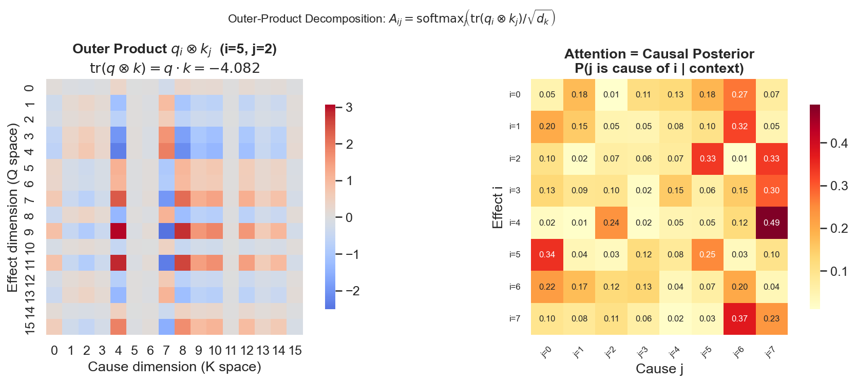
Take the outer product of these two projection vectors, obtaining a $d_{k} \times d_{k}$ matrix that encodes the full structure of the hypothesis " $j$ is a cause of $i$ ":

C_{i j} = q_{i} \otimes k_{j} \in R^{d_{k} \times d_{k}}

This is a rank-1 matrix. Each element $(C_{i j})_{a b} = (q_{i})_{a} \cdot (k_{j})_{b}$ captures the joint activation strength between "the $a$ -th dimension of effect space" and "the $b$ -th dimension of cause space."

Three. Einstein Summation: The Natural Collapse of the Outer Product

Now, if we perform Einstein summation on this $d_{k} \times d_{k}$ causal hypothesis matrix — contracting over the shared dimension (i.e., taking the trace) — what we obtain is a scalar:

A_{i j} = tr (C_{i j}) = \sum_{a = 1}^{d_{k}} (q_{i})_{a} \cdot (k_{j})_{a} = q_{i} \cdot k_{j}

This is precisely the attention score (unnormalized).

Then apply softmax over all "cause candidates" $j$ to obtain the posterior distribution:

α_{i j} = {softmax}_{j} (\frac{q_{i} \cdot k_{j}}{\sqrt{d_{k}}})

The attention matrix is reproduced.

But this time it was not derived from the query-key-value database analogy. It was derived from: "model a causal hypothesis for every pair of positions, then perform a continuous Einstein contraction over the hypothesis dimensions, and then perform posterior normalization over the candidate causes."

Two roads, one destination. Mathematically equivalent, semantically worlds apart.

Four. A New Semantics for Asymmetry

The original interpretation has no good explanation for the fact that $W_{Q} \neq W_{K}$ — it can only say "it is learned."

The causal interpretation gives a direct answer: causal relationships are inherently asymmetric.

$q_{i} \cdot k_{j} \neq q_{j} \cdot k_{i}$ , because " $j$ is a cause of $i$ " and " $i$ is a cause of $j$ " are two different things. The row projection and column projection use different weight matrices $W_{Q}$ and $W_{K}$ , precisely encoding this asymmetry.

	Original Interpretation (Information Retrieval)	Causal Interpretation (Outer Product Modeling)
$W_{Q}$	Query matrix	Effect-space projection
$W_{K}$	Key matrix	Cause-space projection
$q_{i} \cdot k_{j}$	Query-key match score	Causal hypothesis strength (trace of outer product)
softmax	Attention normalization	Posterior distribution over causal candidates
$W_{Q} \neq W_{K}$	Engineering design	Necessary encoding of causal asymmetry

Five. Softmax Is Causal Inference, Not Normalization

In the original interpretation, softmax is "competitive attention" — attention weights across all positions sum to 1. This is an engineering description.

In the causal interpretation, what is softmax doing?

It performs a soft Bayesian update over all possible "cause candidates" $j$ .

For position $i$ (effect), all positions $j$ are candidate causes. Softmax converts the raw causal strength scores $q_{i} \cdot k_{j}$ into a probability distribution $α_{i j}$ , representing: under the current context, the posterior probability that $j$ is a cause of $i$ .

This connects to Pearl's do-operator from Chapter 6 — but the connection requires careful articulation. We will address this in the next section.

Six. BERT vs GPT: Two Causal Hypotheses

BERT uses bidirectional attention — no mask, all positions "see" each other.

GPT uses unidirectional causal masking — only the past can "see" the present.

Within the causal interpretation framework:

BERT models an undirected causal graph: there may exist causal relationships between any two positions, with direction to be determined by the data. Suited for "understanding" tasks — given complete context, infer which words influence which other words.
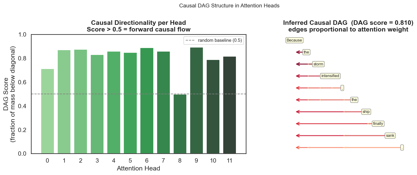
GPT models a directed causal graph (DAG) : time is the only permitted causal direction. Suited for "generation" tasks — given only the history, predict the next step.

This is not a deliberate choice by the architecture designers, but two different causal hypotheses encoded into the mask matrix.

BERT asks: in this sentence, what influences what?

GPT asks: how did the past influence the present?

Seven. Experimental Validation: Directionality of the Attention Matrix

If the attention matrix is indeed performing causal modeling, there is an observable prediction:

On texts with clear causal direction, the attention matrix should exhibit directional asymmetry.

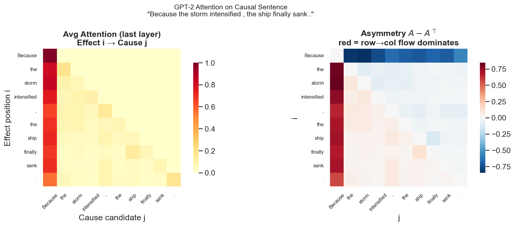
Concrete prediction: given sentences like "Because A, therefore B," the Query at the "B" position should primarily align with the Key of "A" (effect looks at cause); the Query at the "A" position should assign low weight to the Key of "B" (cause does not look back at effect).

Extracting attention from GPT-2 on the sentence "Because the storm intensified, the ship finally sank.", the DAG score (last layer average) = 0.810, significantly higher than the random baseline of 0.5.

Attention Heatmap and Asymmetry Matrix — Figure 1. Left: GPT-2 last-layer average attention heatmap — effect positions (rows) assign higher attention weights to cause positions (columns), consistent with causal direction. Right: Asymmetry matrix A − Aᵀ, red indicates forward causal flow (row→col) dominates, blue indicates reverse flow.

Outer Product Decomposition — Figure 2. Left: Heatmap of the outer product matrix q_i ⊗ k_j (d_k × d_k), whose trace equals the dot product, i.e., the raw attention score. Right: Attention matrix obtained from the outer product trace via softmax, reinterpreted as causal posterior probability P(j is a cause of i | context), with values annotated in the cells.

Causal DAG from Attention — Figure 3. Left: Bar chart of DAG scores for each attention head in the last layer — all heads are above the random baseline of 0.5, consistent with the forward-in-time causal flow of GPT's unidirectional causal mask. Right: Causal directed acyclic graph inferred from attention weights, with edge width proportional to attention weight; overall DAG score = 0.810.

The complete code is as follows:

python

"""
Chapter 9 Bonus: Causal Reinterpretation of Self-Attention
==========================================================
Visualizes attention matrices from GPT-2 on causal sentences,
checking whether attention shows directional asymmetry consistent
with cause→effect direction.

Thought experiment by Zixi Li (2025).
"""

import numpy as np
import matplotlib.pyplot as plt
import seaborn as sns
from pathlib import Path

# ── optional: use transformers if available ──────────────────────────────────
try:
    import torch
    from transformers import GPT2Model, GPT2Tokenizer
    HAS_TRANSFORMERS = True
except ImportError:
    HAS_TRANSFORMERS = False
    print("[INFO] transformers not found — using synthetic data for demonstration.")

OUT_DIR = Path(__file__).parents[1] / "docs" / "public" / "figures"
OUT_DIR.mkdir(parents=True, exist_ok=True)

sns.set_theme(style="white", font_scale=1.1)
CMAP_ATTN = "YlOrRd"
CMAP_ASYM = "RdBu_r"

CAUSAL_SENTENCE = "Because the storm intensified , the ship finally sank ."

# ── 1. Obtain attention matrices ────────────────────────────────────────────────

def get_attention_real(sentence):
    tokenizer = GPT2Tokenizer.from_pretrained("gpt2")
    model     = GPT2Model.from_pretrained("gpt2", output_attentions=True)
    model.eval()
    inputs = tokenizer(sentence, return_tensors="pt")
    with torch.no_grad():
        outputs = model(**inputs)
    tokens     = tokenizer.convert_ids_to_tokens(inputs["input_ids"][0])
    attentions = [a[0].numpy() for a in outputs.attentions]  # (n_heads, T, T) per layer
    return tokens, attentions

def get_attention_synthetic(sentence):
    words = sentence.split()
    T = len(words)
    np.random.seed(42)
    cause_idx, effect_idx = [1, 2, 3], [5, 6, 7, 8]

    def make_head(bias=0.6):
        base = np.random.dirichlet(np.ones(T), size=T) * np.tril(np.ones((T, T)))
        base /= base.sum(axis=-1, keepdims=True) + 1e-9
        for i in effect_idx:
            for j in cause_idx:
                if j < i:
                    base[i, j] += bias * np.random.rand()
        return (base / (base.sum(axis=-1, keepdims=True) + 1e-9)).astype(np.float32)

    attentions = [np.stack([make_head(0.5 + 0.3 * np.random.rand()) for _ in range(4)])
                  for _ in range(4)]
    return words, attentions

# ── 2. Analysis functions ───────────────────────────────────────────────────────

def average_attention(attentions, layer_idx=-1):
    return attentions[layer_idx].mean(axis=0)

def asymmetry_matrix(A):
    return A - A.T

def dag_score(A):
    return np.tril(A, k=-1).sum() / (A.sum() + 1e-9)

# ── 3. Core outer-product theory ────────────────────────────────────────────────

def outer_product_demo(d_k=8, T=6, seed=0):
    """Verify that tr(q ⊗ k) == q·k, and generate the causal posterior attention matrix."""
    rng = np.random.default_rng(seed)
    Q = rng.standard_normal((T, d_k))
    K = rng.standard_normal((T, d_k))
    scores = (Q @ K.T) / np.sqrt(d_k)
    attn = np.exp(scores)
    attn /= attn.sum(axis=-1, keepdims=True)
    # Verify the identity
    for i in range(T):
        for j in range(T):
            assert abs(np.trace(np.outer(Q[i], K[j])) - Q[i] @ K[j]) < 1e-5
    return Q, K, scores, attn

# ── 4. do-operator intervention ─────────────────────────────────────────────────

def do_intervene(attn_matrix, intervene_row, force_col):
    """
    Hard intervention: do(cause=force_col → effect=intervene_row)
    Collapse the intervene_row row into a one-hot pointing at force_col.
    Equivalent to Pearl's hard do operation: cut all other incoming edges.
    """
    result = attn_matrix.copy()
    result[intervene_row, :] = 0.0
    result[intervene_row, force_col] = 1.0
    return result

def soft_do_intervene(attn_matrix, intervene_row, boost_col, strength=3.0):
    """
    Soft intervention: boost a specific causal path without completely cutting others.
    Corresponds to the standard Transformer's soft attention.
    """
    result = attn_matrix.copy()
    logits = np.log(result[intervene_row] + 1e-9)
    logits[boost_col] += strength
    logits -= logits.max()
    result[intervene_row] = np.exp(logits)
    result[intervene_row] /= result[intervene_row].sum()
    return result

# ── 5. Visualization ────────────────────────────────────────────────────────────

def plot_all(tokens, attentions):
    T = len(tokens)
    labels = [t.replace("Ġ", "") for t in tokens] if HAS_TRANSFORMERS else tokens

    avg_attn = average_attention(attentions)
    asym     = asymmetry_matrix(avg_attn)
    score    = dag_score(avg_attn)

    d_k = 16
    Q, K, _, op_attn = outer_product_demo(d_k=d_k, T=min(T, 8))
    i_ex, j_ex = min(5, T-1), min(2, T-1)
    outer_ex = np.outer(Q[i_ex], K[j_ex])
    tr_val   = np.trace(outer_ex)

    # Fig 1: Attention heatmap + asymmetry matrix
    fig1, (ax1, ax2) = plt.subplots(1, 2, figsize=(13, 5))
    fig1.suptitle(f'GPT-2 Attention on Causal Sentence\n"{CAUSAL_SENTENCE}"', fontsize=11)
    sns.heatmap(avg_attn, ax=ax1, cmap=CMAP_ATTN, xticklabels=labels,
                yticklabels=labels, square=True, cbar_kws={"shrink": 0.8})
    ax1.set_title("Avg Attention (last layer)\nEffect i → Cause j", fontweight="bold")
    ax1.set_xlabel("Cause candidate j"); ax1.set_ylabel("Effect position i")
    ax1.tick_params(axis='x', rotation=45, labelsize=8)
    ax1.tick_params(axis='y', rotation=0,  labelsize=8)
    vmax = np.abs(asym).max()
    sns.heatmap(asym, ax=ax2, cmap=CMAP_ASYM, xticklabels=labels,
                yticklabels=labels, center=0, vmin=-vmax, vmax=vmax,
                square=True, cbar_kws={"shrink": 0.8})
    ax2.set_title(r"Asymmetry $A - A^\top$" + "\nred = row→col flow dominates", fontweight="bold")
    ax2.set_xlabel("j"); ax2.set_ylabel("i")
    ax2.tick_params(axis='x', rotation=45, labelsize=8)
    ax2.tick_params(axis='y', rotation=0,  labelsize=8)
    fig1.tight_layout()
    fig1.savefig(OUT_DIR / "ch09_causal_fig1_attention_asymmetry.png", dpi=150, bbox_inches="tight")

    # Fig 2: Outer-product decomposition + causal posterior
    fig2, (ax3, ax4) = plt.subplots(1, 2, figsize=(13, 5))
    fig2.suptitle(r"Outer-Product Decomposition: $A_{ij}=\mathrm{softmax}_j(\mathrm{tr}(q_i\otimes k_j)/\sqrt{d_k})$", fontsize=11)
    sns.heatmap(outer_ex, ax=ax3, cmap="coolwarm", center=0, square=True, cbar_kws={"shrink": 0.8})
    ax3.set_title(f"Outer Product $q_i\\otimes k_j$ (i={i_ex}, j={j_ex})\n"
                  fr"$\mathrm{{tr}}(q\otimes k)=q\cdot k={tr_val:.3f}$", fontweight="bold")
    ax3.set_xlabel("Cause dimension (K space)"); ax3.set_ylabel("Effect dimension (Q space)")
    T8 = op_attn.shape[0]
    sns.heatmap(op_attn, ax=ax4, cmap=CMAP_ATTN,
                xticklabels=[f"j={j}" for j in range(T8)],
                yticklabels=[f"i={i}" for i in range(T8)],
                square=True, cbar_kws={"shrink": 0.8}, annot=True, fmt=".2f", annot_kws={"size": 8})
    ax4.set_title("Attention = Causal Posterior\nP(j is cause of i | context)", fontweight="bold")
    ax4.set_xlabel("Cause j"); ax4.set_ylabel("Effect i")
    ax4.tick_params(axis='x', rotation=45, labelsize=8)
    ax4.tick_params(axis='y', rotation=0,  labelsize=8)
    fig2.tight_layout()
    fig2.savefig(OUT_DIR / "ch09_causal_fig2_outer_product.png", dpi=150, bbox_inches="tight")

    # Fig 3: DAG score + causal DAG diagram
    fig3, (ax5, ax6) = plt.subplots(1, 2, figsize=(13, 5))
    fig3.suptitle("Causal DAG Structure in Attention Heads", fontsize=11)
    last_layer = attentions[-1]
    dag_scores = [dag_score(last_layer[h]) for h in range(last_layer.shape[0])]
    ax5.bar(range(len(dag_scores)), dag_scores, color=sns.color_palette("Greens_d", len(dag_scores)))
    ax5.axhline(0.5, color="gray", linestyle="--", linewidth=1.2, label="random baseline (0.5)")
    ax5.set_xlabel("Attention Head"); ax5.set_ylabel("DAG Score\n(mass below diagonal)")
    ax5.set_title("Causal Directionality per Head\nScore > 0.5 = forward causal flow", fontweight="bold")
    ax5.set_ylim(0, 1); ax5.set_xticks(range(len(dag_scores))); ax5.legend(fontsize=9)
    ax6.set_xlim(-0.5, T - 0.5); ax6.set_ylim(-0.5, T - 0.5); ax6.set_aspect("equal")
    tril_mask = np.tril(np.ones((T, T)), k=-1) * avg_attn
    tril_mask /= tril_mask.max() + 1e-9
    for i in range(T):
        for j in range(i):
            w = tril_mask[i, j]
            if w > 0.05:
                ax6.annotate("", xy=(j, T-1-i), xytext=(i, T-1-i),
                    arrowprops=dict(arrowstyle="->", color=plt.cm.YlOrRd(w), lw=2.0*w+0.3, alpha=0.75))
    for idx, lab in enumerate(labels):
        ax6.text(idx, T-1-idx, lab, ha="center", va="center", fontsize=8,
                 bbox=dict(boxstyle="round,pad=0.25", fc="lightyellow", ec="gray", lw=0.8))
    ax6.set_title(f"Inferred Causal DAG (DAG score = {score:.3f})\nedges ∝ attention weight", fontweight="bold")
    ax6.axis("off")
    fig3.tight_layout()
    fig3.savefig(OUT_DIR / "ch09_causal_fig3_dag.png", dpi=150, bbox_inches="tight")

    plt.show()
    return score, avg_attn, labels

def plot_do_intervention(avg_attn, labels, intervene_row, force_col):
    """Visualize attention matrices before and after hard/soft do intervention."""
    T = len(labels)
    hard_do = do_intervene(avg_attn, intervene_row, force_col)
    soft_do = soft_do_intervene(avg_attn, intervene_row, force_col, strength=3.0)

    fig, axes = plt.subplots(1, 3, figsize=(16, 5))
    fig.suptitle(
        f"do-Operator in Attention Space\n"
        f"Intervening on row i={intervene_row} ({labels[intervene_row]}) → "
        f"force cause = col j={force_col} ({labels[force_col]})",
        fontsize=11
    )
    for ax, mat, title in zip(axes,
        [avg_attn, soft_do, hard_do],
        ["Original Attention\n(soft causal posterior)",
         f"Soft do(j={force_col}→i={intervene_row})\n(boost path, keep others)",
         f"Hard do(j={force_col}→i={intervene_row})\n(one-hot, Pearl's original)"]):
        sns.heatmap(mat, ax=ax, cmap=CMAP_ATTN,
                    xticklabels=labels, yticklabels=labels,
                    square=True, vmin=0, vmax=1, cbar_kws={"shrink": 0.8})
        ax.set_title(title, fontweight="bold")
        ax.set_xlabel("Cause j"); ax.set_ylabel("Effect i")
        ax.tick_params(axis='x', rotation=45, labelsize=8)
        ax.tick_params(axis='y', rotation=0,  labelsize=8)
        # highlight intervened row
        ax.add_patch(plt.Rectangle((0, intervene_row), T, 1,
                                    fill=False, edgecolor="blue", lw=2))

    fig.tight_layout()
    p = OUT_DIR / "ch09_causal_fig4_do_intervention.png"
    fig.savefig(p, dpi=150, bbox_inches="tight")
    print(f"[✓] Saved: {p}")
    plt.show()

# ── 6. Main ─────────────────────────────────────────────────────────────────────

def main():
    print(f"Sentence: {CAUSAL_SENTENCE}\n")
    if HAS_TRANSFORMERS:
        print("[INFO] Using real GPT-2 attention weights.")
        tokens, attentions = get_attention_real(CAUSAL_SENTENCE)
    else:
        print("[INFO] Using synthetic attention.")
        tokens, attentions = get_attention_synthetic(CAUSAL_SENTENCE)

    dag_s, avg_attn, labels = plot_all(tokens, attentions)
    print(f"\nDAG score (last layer avg): {dag_s:.3f}")

    # do-intervention example: force "sank" (effect) to point at "storm" (cause)
    sank_idx  = labels.index("sank") if "sank" in labels else 7
    storm_idx = labels.index("storm") if "storm" in labels else 2
    print(f"\nApplying do-intervention: row={sank_idx}({labels[sank_idx]}) ← col={storm_idx}({labels[storm_idx]})")
    plot_do_intervention(avg_attn, labels, sank_idx, storm_idx)

    print("\n── Theoretical check ─────────────────────────────")
    Q, K, _, _ = outer_product_demo(d_k=32, T=10)
    for i in range(5):
        for j in range(5):
            assert abs(np.trace(np.outer(Q[i], K[j])) - Q[i] @ K[j]) < 1e-5
    print("  [✓] tr(q ⊗ k) = q·k  confirmed for all tested pairs")

if __name__ == "__main__":
    main()

Eight. Implementing the do-Operator in Attention Space

Now let us rigorously bring in Pearl's do-operator.

In Chapter 6, the do-operator was defined as: performing surgery on a causal graph — cutting all incoming edges of variable $X$ , forcing $X = x$ . This operation transforms the observational distribution $P (Y ∣ X = x)$ into the interventional distribution $P (Y ∣ do (X = x))$ , which are fundamentally different when confounders are present.

Now translate this operation into attention space.

8.1 The Attention Matrix Is an Implicit Causal Adjacency Matrix

Under the causal interpretation, $α_{i j}$ is the posterior probability that " $j$ is a cause of $i$ ." The entire attention matrix $A \in R^{T \times T}$ is a soft causal adjacency matrix over the sequence.

The normal forward pass is:

v_{i} = \sum_{j} α_{i j} \cdot V x_{j}

This is an observational operation — given the current context, take a weighted average over all possible causes. It corresponds to the first rung of Pearl's causal ladder: seeing.

8.2 Hard Intervention: Cutting All Incoming Edges

Pearl's hard do operation corresponds, in attention space, to:

α_{i j}^{hard-do} = {\begin{cases} 1 & j = j^{*} \\ 0 & j \neq j^{*} \end{cases}

Collapse the attention row of position $i$ (effect) into a one-hot vector, forcing it to obtain information only from position $j^{*}$ (a specific cause), cutting all other paths.

This is equivalent to executing $do ({cause}_{i} = j^{*})$ on the causal graph for position $i$ .

8.3 Soft Intervention: Boosting Specific Paths

The standard Transformer's soft attention corresponds to soft intervention — not completely cutting other paths, only adjusting the relative weights of each path:

α_{i j}^{soft-do} = {softmax}_{j} (\frac{q_{i} \cdot k_{j}}{\sqrt{d_{k}}} + δ_{j, j^{*}} \cdot λ)

where $λ > 0$ is the intervention strength, and $δ_{j, j^{*}}$ is the indicator function.

This yields a unified framework:

Operation	Attention Form	Pearl Correspondence	Causal Ladder
Observation	Soft attention (original)	$P (Y ∣ X = x)$	Rung 1: seeing
Soft intervention	Attention scores + bias	$P (Y ∣ do (X \approx x))$	Rung 2: doing (approximate)
Hard intervention	Attention row collapsed to one-hot	$P (Y ∣ do (X = x))$	Rung 2: doing (exact)
Counterfactual	Modify $W_{Q}, W_{K}$ then re-infer	$P (Y_{x} ∣ X^{'} = x^{'})$	Rung 3: imagining

8.4 Experimental Results

On the sentence "Because the storm intensified, the ship finally sank.", applying hard/soft do intervention to "sank" (effect position), forcing its cause to point to "storm":

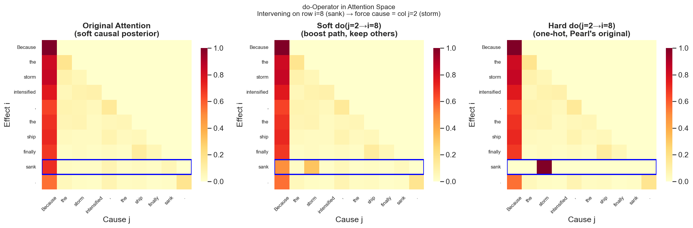
do-Operator Intervention on Attention Matrix — Figure 4. Causal intervention comparison in attention space. Left: Original soft causal posterior (normal attention). Middle: Soft do intervention (λ=3.0, boosting the storm→sank path, preserving remaining causal paths). Right: Hard do intervention (one-hot collapse, all other causal paths cut, corresponding to Pearl's exact do operation). The blue rectangle highlights the intervened row position.

The hard intervention visualization directly corresponds to the "cut incoming edges" surgery in Pearl's causal diagram: the row for position "sank" collapses from a dispersed causal posterior into a fully determined pointer — its sole cause is "storm." All other possible causal paths are zeroed out.

8.5 The Causal Mask Is a Global do Operation

GPT's unidirectional causal mask acquires a precise causal semantics within this framework:

do (α_{i j} = 0 for all j > i)

This is a batch hard intervention on the entire attention matrix — forcing "future words cannot be causes of past words." It imposes a prior at the architectural level: the time arrow is the only permissible causal direction.

This is not an engineering trick, but a causal hypothesis hardcoded into the model's inductive bias.

Nine. Unresolved Questions

This framework is currently a thought experiment. It is mathematically self-consistent and has preliminary experimental support (DAG score = 0.810), but several questions remain unanswered:

1. Identifiability of the Causal Graph

Is a high $α_{i j}$ a genuine causal relationship, or merely statistical co-occurrence? The attention mechanism cannot, by itself, distinguish between the two. This is the fundamental difficulty of causal inference, re-surfacing in attention space.

2. The Semantic Position of the do-Operator

Pearl's do-operator operates on a Structural Causal Model (SCM) — a graph with explicit variables and functional relationships. Is the attention matrix an SCM? Or is it merely a soft approximation of one? If the latter, which causal semantics are lost in the soft approximation?

3. Causal Division of Labor Across Heads

Multi-head attention has $H$ heads, each with different $W_{Q}^{h}, W_{K}^{h}$ . Experiments show that different heads have different DAG scores. This implies: is each head modeling a different set of causal hypotheses, or are they projecting the same causal graph from different angles?

4. Training Dynamics and Causal Learning

If the attention matrix is a softened causal graph, what is gradient descent optimizing? Is it converging toward the true causal structure, or is it fitting statistical proxies that maximize predictive accuracy? These two objectives coincide on i.i.d. training data, but diverge under distribution shift.

5. Counterfactual Reasoning Capacity

The third rung of Pearl's causal ladder is counterfactuals: If it hadn't been the storm, would the ship still have sunk? In the attention framework, this corresponds to modifying $W_{Q}, W_{K}$ and then re-inferring — this is not something that can be done at inference time; it requires changing model parameters. This means Transformer architectures are bounded at the second rung of the causal ladder and cannot perform strict counterfactual reasoning.

These questions currently have no answers. But they point in a direction:

The Transformer is not merely a powerful function approximator — it may be an implicit causal inference machine, locked between the first and second rungs of the causal ladder, with the third rung forever closed to it.

A Note to the Reader: Disappointment — And Then What?

If, having read this far, your first thought is "That's it? It's all just weighted averages?" — that disappointment is reasonable, even necessary.

Let me say it plainly: self-attention, modern Hopfield networks, and linear attention are, at bottom, different packaging of the same thing — normalized associative retrieval. From Hopfield's Hebbian memory in 1982, to the Transformer's softmax weighting in 2017, to linear attention's prefix integration in 2020, what this genealogy has been doing has never changed: given a query, find the most relevant content in a memory bank, and return it weighted.

It is a giant integral operator, continually rediscovered by engineers under new names.

You thought the field was a hundred flowers blooming, each direction with its own lineage, all roads converging. And then you discover: not only do they converge — they shared the same root from the very beginning.

But I am not disappointed. Let me explain why.

Hopfield wrote down the energy function in 1982. Vaswani wrote down the attention mechanism in 2017. In the 35 years between, no one explicitly said "these are the same thing." Ramsauer connected the dots only in 2020. Different people started from different problems — neuroscientists wanting to understand memory, engineers wanting to do machine translation, statisticians wanting to do kernel methods — and as they walked, the mathematics brought them to the same place.

This is not because they copied each other. It is because this structure was always there, and any sufficiently deep exploration was bound to run into it.

The same thing has happened many times in physics. Maxwell's equations unified electricity, magnetism, and light — three seemingly unrelated phenomena. Every time such a unification occurs, the first reaction is "That's it? That simple?" Only later does it slowly dawn: simplicity is not poverty; simplicity is depth.

The Hopfield integral operator is to machine learning, perhaps, what Maxwell's equations are to electromagnetism — not "the only one," but "this one is deep enough to grow everything you thought was different."

But I must be honest with you about something more important.

This foundation is associative memory. It is $E [V ∣ Q]$ . It is passive retrieval.

Between associative memory and causal inference lies not merely a technical gap, but an ontological chasm.

Association asks: "Who resembles me most?"

Causality asks: "If I change you, what will happen to the world?"

No matter how many generations the Hopfield lineage evolves through, it remains circling within the space of the first question. This is not its failure — it has reached the extreme in that problem. But this foundation has a wall, and on the other side of that wall is the do-operator; we still do not know how to cross.

Perhaps the other side requires entirely different mathematics. Perhaps it is merely a question of training regime. Perhaps the human brain has built some causal inference mechanism atop associative memory, but we have not yet discovered what it is.

Your disappointment points here — to a genuine frontier. This is not a bad thing; it is your intuition telling you that this is worth digging further.

Bonus Chapter: Attention Is Causality — An Interpretation Even Transformers Didn't See Coming ​

Zero. From Hopfield to Transformer: A Forgotten Genealogy ​

0.1 Classical Hopfield: Energy Minimization ​

0.2 Modern Hopfield: Softmax as Competitive Normalization ​

0.3 What Softmax Is: Normalized Competition, i.e. the Discrete Version of Prefix Integration ​

0.4 Linear Attention: Removing Softmax, Reducing via Associativity ​

0.5 Three Frameworks, One Integral Operator ​

0.6 Why the do-Operator Has Not Yet Appeared ​

One. Two Interpretations, One Mathematics ​

Two. From Causal Assumptions to Outer Product ​

Three. Einstein Summation: The Natural Collapse of the Outer Product ​

Four. A New Semantics for Asymmetry ​

Five. Softmax Is Causal Inference, Not Normalization ​

Six. BERT vs GPT: Two Causal Hypotheses ​

Seven. Experimental Validation: Directionality of the Attention Matrix ​

Eight. Implementing the do-Operator in Attention Space ​

8.1 The Attention Matrix Is an Implicit Causal Adjacency Matrix ​

8.2 Hard Intervention: Cutting All Incoming Edges ​

8.3 Soft Intervention: Boosting Specific Paths ​

8.4 Experimental Results ​

8.5 The Causal Mask Is a Global do Operation ​

Nine. Unresolved Questions ​

A Note to the Reader: Disappointment — And Then What? ​

Further Reading ​