Chapter 9: Transformer: The Attention Revolution of Dynamic Topology

Every Attention Head is asking: at this moment, which parts are important to which parts?

---

I. A Paper in June 2017

On June 12, 2017, eight authors led by Ashish Vaswani of Google Brain uploaded a paper to arXiv with the title "Attention Is All You Need."

The title was audacious. At the time, the dominant architecture for machine translation was RNNs (Recurrent Neural Networks) and LSTMs (Long Short-Term Memory networks)—they had ruled the NLP field for over twenty years. And this paper said: you are all unnecessary; attention mechanism alone is enough.

More audaciously, they were right.

Five months later, the paper was accepted by NIPS 2017. Two years later, BERT and GPT-2 burst onto the scene, all based on the Transformer architecture. Three more years later, GPT-3 proved that Transformers could scale to 175 billion parameters.

Today, virtually all large language models—from ChatGPT to Claude—are variants of the Transformer.

But in June 2017, it was just a radical idea: could we completely abandon recurrent structures?

1.1 The Cost of Sequential Dependency

RNNs work in a very intuitive way: process words one by one from left to right, at each step combining the current word with the previous "memory" to update the hidden state.

$$h_t=f(h_{t-1},x_t)$$

This design looks very natural—after all, humans also read sentences from left to right. But it has two fatal flaws:

RNN, LSTM: What are Recurrent Neural Networks?

RNN (Recurrent Neural Network): A neural network that processes sequences by time steps. At each step, it receives the current input $x_t$ and the hidden state $h_{t-1}$ from the previous step, and outputs a new hidden state $h_t$. Because the hidden state is "recurrently" passed between steps, it is called "recurrent."

Intuitive analogy: each time you read a word, you update your mental understanding of the sentence, then read the next word—RNNs simulate this process.

LSTM (Long Short-Term Memory): An improved version of RNNs, adding "gating" mechanisms (forget gate, input gate, output gate) to control which information should be retained and which should be forgotten, mitigating the problem of long-distance information loss.

Vanishing gradient: When training neural networks, the error signal (gradient) propagates from the output layer to the input layer. If the propagation path is very long (e.g., an RNN processing a long sentence), the gradient gets repeatedly multiplied by numbers less than 1, eventually becoming close to zero—distant weights then "cannot learn anything." LSTMs mitigate this problem through gating, but do not fundamentally solve it.

Flaw 1: Inability to parallelize

To compute the hidden state of the 10th word, you must first compute the hidden state of the 9th word; to compute the 9th word's, you must first compute the 8th word's... This chain cannot be parallelized.

In the GPU era, this is catastrophic. GPUs have thousands of cores and can simultaneously compute thousands of operations. But RNNs force you to compute serially—processing only one word at a time.

For a sequence of length N, an RNN requires N steps of serial computation. Even if each step takes only 1 millisecond, a sentence of 1000 words would take 1 second.

Flaw 2: Information decay in long-range dependencies

Suppose you want to translate this sentence:

"The cat, which we found in the garden last summer, was very friendly."

The subject "cat" and the predicate "was" are separated by 12 words. The RNN needs to pass the information of "cat" through 12 steps to reach "was."

With each step of transmission, information decays. Even with LSTM's gating mechanisms, long-distance transmission remains difficult—this is another manifestation of the vanishing gradient problem.

Bengio et al. proved in 1994: when RNNs learn long-range dependencies, gradients decay exponentially. LSTMs mitigate this problem but do not fundamentally solve it.

1.2 Vaswani's Wager

The idea of Vaswani et al. was: if every word could directly "see" all other words, there would be no need to pass information through hidden states.

This is the Self-Attention mechanism. It allows every position in a sequence to directly compute its relevance to all other positions, then perform a weighted sum using those relevance scores.

No recurrence, no sequential dependency, fully parallelizable computation.

What is the cost? Computational complexity goes from $O(N)$ to $O(N^2)$.

Self-Attention: Every word asks every other word, "Are you important?"

The core idea of Self-Attention: when processing a sentence, for each word, let it "query" all other words in the sentence "How important are you to me?", then combine information from all words weighted by importance.

Intuitive example: "The bank failed"—when processing the word "failed," Self-Attention lets "failed" ask "bank," "The" etc. about their importance, discovers that "bank" is most relevant, and thus references "bank"'s information more heavily to understand the context of "failed."

The $O(N^2)$ cost: With sequence length $N$, each word must compute relevance with all $N$ other words, totaling $N\times N=N^2$ computations. When $N=1000$, that's 1 million; when $N=10000$, that's 100 million. This is why long context windows are expensive.

Why is it worth it? Because all $N^2$ computations can be fully parallelized—GPUs process them simultaneously, while an RNN's $N$ steps can only be serial. Total time is actually shorter, and there is no information decay problem.

For a sequence of length N, Self-Attention requires computing an $N\times N$ attention matrix—the relevance of every word to every other word. When N=512, that's 262,144 numbers. When N=2048, that's 4,194,304 numbers.

This is a bold wager: trade $O(N^2)$ space and computation for parallelization and a global receptive field.

The results proved this wager was worthwhile.

---

A Pause

"The results proved this wager was worthwhile"—but worthwhile, by what measure?

Does the Transformer work because Self-Attention, as a design, is structurally closer to the "true structure" of language than RNNs? Or is it simply because $O(N^2)$ computation is more easily exploited by GPU parallelism, allowing it to use more data and compute to compensate for architectural deficiencies?

In other words: Is the Transformer's success due to its inductive bias being correct, or due to its inductive bias being the weakest—so weak that brute-force data can fill the gap?

"Having no inductive bias" is itself an inductive bias. The Transformer assumes that "words at any position may be important to words at any other position." Is this assumption correct for language? Is it correct for all tasks?

Set this question aside for now.

---

II. The Mathematics of Self-Attention: An Elegant Symmetry

The core of the Transformer is the Self-Attention mechanism. The problem it aims to solve is simple:

Given a sequence, how can every position "see" all other positions, and decide which positions are important?

The mathematical form is surprisingly concise. For an input sequence $X\in {\mathbb{R}}^{N\times d}$ (N words, each word d-dimensional), compute three matrices:

$$Q=X{W}_Q,K=X{W}_K,V=X{W}_V$$

These three matrices have different semantic roles:

• Query: "What am I looking for?"—the pattern the current position wants to attend to

• Key: "What can I provide?"—the index information each position offers

• Value: "What is my content?"—the actual information at each position

Then compute attention:

$$\text{Attention}(Q,K,V)=\text{softmax}\left(\frac{Q{K}^T}{\sqrt{d_k}}\right)V$$

Let me unpack every step of this formula:

Step 1: Compute similarity $Q{K}^T\in {\mathbb{R}}^{N\times N}$

Each query takes the dot product with each key. The element at row $i$, column $j$ is $q_i\cdot k_j$—representing position $i$'s "degree of interest" in position $j$.

Why can the dot product measure similarity? Because $q\cdot k=|q||k|\cos \theta$—when two vectors point in the same direction, the dot product is maximized.

Step 2: Scale Divide by $\sqrt{d_k}$

This is a crucial technical detail. When $d_k$ is large, the variance of dot products can be very large—extremely large positive or negative values may appear. This causes the softmax to saturate: the probability for the maximum value approaches 1, and all other positions approach 0.

Under the initialization assumption, each dimension of $Q$ and $K$ is independent with constant variance, so the variance of the dot product $Q\cdot K$ is proportional to dimension $d$. Using $\frac{1}{\sqrt{d_k}}$ for scaling normalizes its variance to a stable range of $O(1)$, thereby preventing $softmax$ from entering saturated or excessively flat regions. During training, although the representation distribution may shift, layer normalization re-normalizes the input distribution, and residual connections stabilize the gradient flow, allowing the model to adaptively maintain the attention score scale within a reasonable range, ensuring training stability.

Step 3: Normalize softmax normalization per row

Convert similarities into a probability distribution. The softmax output of row $i$ is a probability vector summing to 1, representing position $i$'s attention allocation across all other positions.

Step 4: Weighted sum Multiply by $V$

Use the attention weights to compute a weighted sum of values. The output of position $i$ is:

$${\text{out}}_i=\sum _{j=1}^N{\text{attention}}_{ij}\cdot v_j$$

This is a soft addressing mechanism: instead of hard-selecting a specific position, it computes a weighted average over all positions, with weights determined by similarity.

The beauty of this mechanism:

1. Global receptive field: Each position can directly "see" all other positions, without passing through hidden states

2. Fully parallel: All positions' outputs can be computed simultaneously, with no sequential dependency

3. Dynamic topology: The attention matrix is dynamically generated based on input content, not fixed weights

---

III. Hands-On: Seeing What Attention Is "Looking" At

Take out a piece of paper and manually compute a simple example.

Input sentence: "cat sat mat" (3 words, for simplicity)

Assume each word has been embedded as a 2-dimensional vector:

cat: [1, 0]
sat: [0, 1]
mat: [1, 1]

Step 1: Compute Q, K, V

For simplicity, assume $W_Q=W_K=W_V=I$ (identity matrix), so $Q=K=V=X$.

Step 2: Compute attention scores

$$Q{K}^T=\left[\begin{array}{cc}1& 0\\ 0& 1\\ 1& 1\end{array}\right]\left[\begin{array}{ccc}1& 0& 1\\ 0& 1& 1\end{array}\right]=\left[\begin{array}{ccc}1& 0& 1\\ 0& 1& 1\\ 1& 1& 2\end{array}\right]$$

Divide by $\sqrt{d_k}=\sqrt{2}\approx 1.41$:

$$\text{scores}=\left[\begin{array}{ccc}0.71& 0& 0.71\\ 0& 0.71& 0.71\\ 0.71& 0.71& 1.41\end{array}\right]$$

Step 3: Apply softmax (per row)

For the first row $[0.71,0,0.71]$:

$$\text{softmax}=\frac{[e^{0.71},e^0,e^{0.71}]}{\sum }\approx [0.42,0.16,0.42]$$

The complete attention matrix (approximate):

$$A=\left[\begin{array}{ccc}0.42& 0.16& 0.42\\ 0.16& 0.42& 0.42\\ 0.27& 0.27& 0.46\end{array}\right]$$

Interpretation: - Row 1: "cat" has similar attention to itself (0.42) and "mat" (0.42), lower attention to "sat" (0.16) - Row 3: "mat" attends to all words, but highest to itself (0.46)

Step 4: Weighted sum

Output for the 1st word:

$${\text{out}}_1=0.42\times [1,0]+0.16\times [0,1]+0.42\times [1,1]=[0.84,0.58]$$

This vector fuses information from "cat" and "mat," because the attention weights are high.

Key observation: The attention matrix $A$ is dynamically generated—it is not a fixed weight, but computed based on input content. This is the meaning of "dynamic topology."

---

Professor Pallas's Cat's Monologue: The Dynamic Topology of Hidden Space

---

There is a fatal weakness in the textbooks.

They say: "The attention mechanism models explicit relationships between tokens." They say: "Self-Attention lets every token directly see all other tokens."

This is wrong.

Let me clarify a core misconception—one that has even infiltrated papers at many top conferences, leading the entire community down the wrong intuition for years.

Spatial Confusion: Hidden Space vs. Token Space

People always think that attention operates in "token space." But what is "token space"? Is it the lookup table of embedding vectors? That space only encodes word forms; it is static, vocabulary-level.

The real operation occurs in hidden space.

When a sequence $X$ enters the Transformer, it first becomes:

$$X_{\text{hidden}}=\text{LayerNorm}(X_{\text{embed}}+\text{PositionalEncoding})$$

Positional encoding, layer normalization... these are not decorations. They transform static embeddings into context-dependent hidden representations.

Then attention takes the stage:

$$\text{Attention}(Q,K,V)=\text{softmax}\left(\frac{Q{K}^T}{\sqrt{d_k}}\right)V$$

Note: $Q=X_{\text{hidden}}{W}_Q,K=X_{\text{hidden}}{W}_K,V=X_{\text{hidden}}{W}_V$.

$Q,K,V$ are projections of hidden representations, not projections of the tokens themselves.

The Real Operation: Representation Retrieval in Hidden Space

So, what is attention doing?

It is not comparing "token A" with "token B." It is comparing "the hidden representation of position A" with "the hidden representation of position B."

To put it in more technical terms:

• Embedding space: Word form → Static vector
• Hidden space: Contextual understanding → Dynamic vector

The attention mechanism performs representation retrieval within hidden space. $q_i$ is a query: "Given my current contextual understanding, what information do I need?" $k_j$ is an index: "Given my current contextual understanding, what information do I provide?"

The similarity $q_i\cdot k_j$ measures the degree of match between two contextual understandings, not between two words.

RNN's Hard Bottleneck vs. Transformer's Dynamic Topology

This distinction reveals the essence of the two architectures:

RNN: The hard bottleneck of explicit memory recurrence

$$h_t=f(h_{t-1},x_t)$$

• $h_t$ is a fixed-dimensional hidden vector
• All historical information must be compressed into this low-dimensional space
• This is a hard bottleneck—information is forced into dimensionality reduction, like compressing a book into a one-page summary
• Vanishing/exploding gradients are the inevitable cost of this one-dimensional chain structure
• Low-entropy structure: Connection pattern is fixed, information capacity is constant

Transformer: The dynamic topology of hidden space

• Each hidden representation $h_i$ generates $q_i,k_i,v_i$ via QKV projections
• Attention weights ${\alpha }_{ij}$ are computed in real time, forming a dynamic connection graph
• No fixed-dimensional bottleneck—information capacity scales with sequence length
• High-entropy structure: Connection weights are dynamically generated, with extremely high representational degrees of freedom

Entropy and Representational Degrees of Freedom

Let me use slightly more quantitative terminology:

• RNN representational degrees of freedom: $O(d_{\text{hidden}})$, independent of sequence length
• Attention representational degrees of freedom: $O(N\times d_{\text{model}})$, scales linearly with sequence length

But attention is not just "more storage." Its high entropy comes from dynamic selectivity.

For every input, it constructs in real time a topological structure optimally suited to the current context. This adaptivity—building connections on demand within hidden space—is the true manifestation of intelligence.

GPT's Pyramid Structure

This also explains why GPT can still function after pruning some layers.

The Transformer is not a flat structure, but a pyramid:

• Shallow hidden layers: Encode surface syntax, local dependencies
• Middle hidden layers: Encode phrase structure, medium-distance dependencies
• Deep hidden layers: Encode semantic roles, logical relationships, long-range dependencies

Each layer performs "representation refinement" within hidden space. Pruning top layers only loses the most abstract understanding; the foundations in the lower layers remain.

The True Meaning of Dynamic Topology

Now I can define "dynamic topology" more precisely:

The attention mechanism is a dynamic connection graph constructed in real time within hidden space, based on the current context. These connections are not determined by tokens, but by the hidden representations of tokens in specific contexts.

The same word ("bank"):

• In a riverbank context, its hidden representation encodes "river, shore, nature"
• In a financial bank context, its hidden representation encodes "finance, money, commerce"

Therefore, its attention patterns with other words are completely different.

This is the charm of dynamic topology—connections are context-dependent, content-driven, and evolve in real time.

It is not "all tokens equally see all other tokens." Rather, it is "under the current hidden representations, which positions' understandings are most relevant to the current position's understanding."

A Clarification from Graph Theory: Seeing ≠ Walking

But there is an even deeper misconception, especially common in textbooks.

Those books love to use "two kids making friends" as a metaphor for the attention mechanism: each child (token) can see all other children and then decide whose hand to hold. This metaphor is vivid, but misses the most critical link.

Seeing does not equal being able to walk there, nor being able to pass messages.

In the language of graph theory: view one layer of a Transformer as a complete graph, where each node (position) has an edge pointing to all other nodes. This edge represents "attention"—I can see your hidden representation, I can take information from you.

But the "bandwidth" of this edge is limited. A single attention operation is merely a single shallow information integration. If you want to have deep information fusion with a distant node—say, integrating its semantics with your syntax, then further fusing with a third node's pragmatic information—you need multi-step propagation.

In a Transformer, one step is one layer.

Therefore:

• One-layer Transformer: Each position can see all positions, but can only do one shallow integration
• Two-layer Transformer: Information can propagate two steps—A takes information from B, integrates it, then takes information from C
• L-layer Transformer: Information can walk L steps in the graph, achieving deep, multi-hop fusion

This is why depth is so important.

At the same width ($d_{\text{model}}$):

• Shallow networks: Information fusion paths are short; only local or shallow pattern matching is possible
• Deep networks: Information can "travel" farther in hidden space, achieving integration across multiple abstraction levels

The length of information fusion ≈ the depth of the network.

This is not my speculation. This is a basic fact of graph theory: in a graph $G$, the path length from node $u$ to node $v$ determines the number of "hops" information can propagate from $u$ to $v$. The attention mechanism gives you the edges of a complete graph (one step reachable), but true semantic integration requires multi-hop paths.

For example:

• Layer 1: Learn part-of-speech tagging (noun/verb)
• Layer 2: Learn phrase structure (noun phrase/verb phrase)
• Layer 3: Learn syntactic roles (subject/object)
• Layer 4: Learn semantic relations (agent/patient)
• Layer 5: Learn pragmatic intent (statement/question/command)

Each layer performs deeper information fusion on the foundation of the previous layer. Without sufficient depth, information cannot "travel" to sufficiently abstract levels.

So, when you hear "Transformer lets every token see every token," remember:

• It describes the local property of one layer
• True understanding requires the deep propagation paths formed by stacking multiple layers
• This is why GPT-3 has 96 layers, not 1

Seeing is free; walking requires paying the cost of layers.

Returning to That Classic Question

Now we can answer that suspended question:

Is the Transformer's success due to its inductive bias being correct?

The answer is: partially correct.

Its inductive bias is not "all tokens may be relevant," but something deeper:

"In an appropriate hidden space, context-dependent representations can be selectively integrated through dynamic topology."

This bias is closer to the true structure of language than RNN's "sequence is a Markov chain," yet not so weak as to have no bias at all.

It falls precisely on the sweet spot between "flexible enough to capture linguistic complexity" and "biased enough to learn efficiently."

---

"Alright, now we can continue discussing multi-head attention."

---

IV. Multi-Head Attention: Division of Labor and Collaboration

A single attention head can only capture one relational pattern. But relationships in language are diverse:

• Syntactic relations: subject-predicate, modifier-head

• Semantic relations: pronoun-antecedent, synonyms

• Positional relations: adjacent words, long-distance dependencies

The Transformer uses Multi-Head Attention to solve this problem: run multiple attention heads in parallel, each learning a different relational pattern.

$$\text{MultiHead}(Q,K,V)=\text{Concat}({\text{head}}_1,\dots ,{\text{head}}_h)W^O$$

Where each head:

$${\text{head}}_i=\text{Attention}(Q{W}_i^Q,K{W}_i^K,V{W}_i^V)$$

Intuition: Divide the $d$-dimensional space into $h$ subspaces, each $d/h$ dimensions. Each head performs attention within its own subspace, and finally concatenates them together.

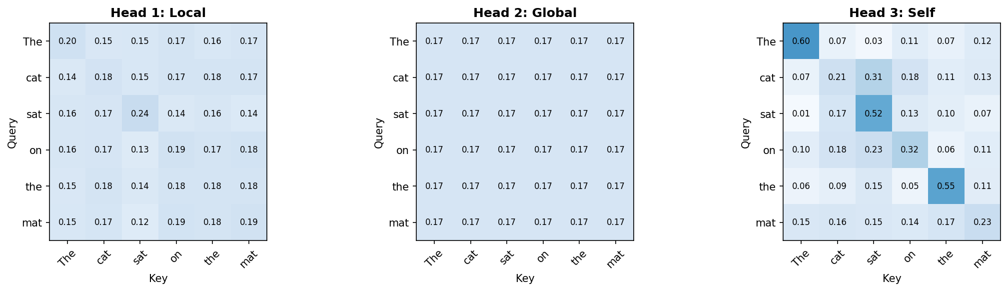
Experimental observations (from BERT visualization studies):

• Head 1: Attends to adjacent words (local syntax)
• Head 2: Attends to pronouns and antecedents (coreference resolution)
• Head 3: Attends to sentence beginnings and endings (global structure)
• Head 4: Attends to punctuation marks (syntactic boundaries)

Different heads spontaneously learned different linguistic functions, despite no explicit supervision.

---

V. The Cost of O(N²): The Thermodynamic Bill of a Global Receptive Field

The time complexity of Self-Attention is $O(N^{2}d)$, and the space complexity is $O(N^2)$.

This is not a constant factor that can be optimized away; it is the intrinsic cost of the architecture.

5.1 Why N²?

Computing $Q{K}^T$ requires $N\times N$ dot products, each requiring $d$ multiplications. Total: $O(N^{2}d)$ operations.

Storing the attention matrix requires $N\times N$ floating-point numbers. When $N=512$, that's 262,144 numbers. When $N=2048$, that's 4,194,304 numbers.

Comparing other architectures:

• RNN: $O(N{d}^2)$ — linear in sequence length, but sequentially dependent

• CNN: $O(Nk{d}^2)$ — linear in sequence length, but receptive field limited by kernel size $k$

• Transformer: $O(N^{2}d)$ — global receptive field, but quadratic complexity

5.2 An Information-Theoretic Perspective: The Entropy Cost of Full Connectivity

From an information-theoretic perspective, $O(N^2)$ complexity is the inevitable consequence of fully-connected topology.

RNN is a chain topology: each node only connects to the previous node. Information flow is unidirectional, left to right. This is a low-entropy structure—the connection pattern is deterministic and does not need to be stored.

Transformer is a fully-connected topology: each node connects to all other nodes. This is a high-entropy structure—connection weights (the attention matrix) are dynamic and must be stored.

Shannon's information theory tells us: describing the connection weights of an $N$-node fully-connected graph requires $\mathrm{\Omega }(N^2)$ bits of information—because there are $N^2$ edges.

This is not an implementation issue; this is an information-theoretic lower bound.

5.3 A Physics Perspective: The Constraint of Landauer's Principle

Landauer's principle states: erasing 1 bit of information requires at least $k_{B}T\ln 2$ of energy.

In every forward pass, the Transformer computes and stores $N^2$ attention weights. On the next token, these weights are "erased" (recomputed).

This means: processing a sequence of length $N$, the Transformer requires at least $O(N^2{k}_{B}T\ln 2)$ of energy—this is the thermodynamic lower bound.

When $N=2048$, at room temperature $T=300K$, this is approximately ${10}^{-18}$ joules. It looks very small, but when you process billions of tokens, this accumulates into significant energy consumption.

GPT-3 training consumed approximately 1287 MWh of electricity. A substantial portion of that was used for computing and storing the attention matrix.

5.4 Is This Cost Worth It?

For sequences of length $<2048$, the answer is yes. Transformers comprehensively surpass RNNs on tasks like machine translation, text generation, and question answering.

But for long sequences (document-level translation, long text summarization, gene sequence analysis), $O(N^2)$ becomes a bottleneck.

This has spawned a series of "efficient Transformer" research efforts:

• Sparse Attention: Only compute partial attention, e.g., local windows + global tokens

• Linear Attention: Use kernel tricks to reduce complexity to $O(N{d}^2)$

• Reformer: Use locality-sensitive hashing to approximate attention

• Longformer: Mix local windows and global attention

But all these methods have a cost: either sacrifice the global receptive field, or introduce approximation error.

No free lunch: global receptive field and linear complexity—you can only pick one. This is not an engineering limitation; this is a fundamental constraint from information theory and thermodynamics.

---

VI. Linear Attention: Replacing softmax with the Associativity of Addition

The root of $O(N^2)$ lies in $Q{K}^T$—this matrix must be fully computed before softmax normalization can be applied to each row.

So, what if we remove softmax?

---

8.1 A Kernel Function Perspective

Recall standard attention:

$${\text{out}}_i=\frac{\sum _j\exp (q_i\cdot k_j)\cdot v_j}{\sum _j\exp (q_i\cdot k_j)}$$

The $\exp (q\cdot k)$ inside softmax can be viewed as a kernel function $\kappa (q,k)$, which measures the similarity between query and key.

Kernel functions have a universal approximation scheme: feature mapping. If there exists a function $\varphi (\cdot )$ such that:

$$\kappa (q,k)\approx \varphi (q{)}^T\varphi (k)$$

Then attention can be rewritten as:

$${\text{out}}_i=\frac{\sum _j\varphi (q_i{)}^T\varphi (k_j)\cdot v_j}{\sum _j\varphi (q_i{)}^T\varphi (k_j)}$$

Key: Using the associativity of addition and matrix multiplication, swap the order of the parentheses:

$${\text{out}}_i=\frac{\varphi (q_i{)}^T(\sum _j\varphi (k_j)v_j^T)}{\varphi (q_i{)}^T(\sum _j\varphi (k_j))}$$

Now the $\sum _j\varphi (k_j)v_j^T$ and $\sum _j\varphi (k_j)$ in the numerator and denominator can be precomputed once and stored as two fixed matrices. The computational cost of these two matrices is $O(N{d}^2)$—linear in sequence length.

All $N$ queries share these two matrices; each query's computation is a single matrix-vector multiplication, costing $O(d^2)$.

Total complexity: $O(N{d}^2)$. Linear attention is born.

---

8.2 The Fatal Flaw of Linear Attention: Smoothness

This sounds perfect. But linear attention has consistently underperformed standard attention in practice—especially when precise, sharp attention is needed (e.g., coreference resolution, keyword matching).

The reason is: softmax naturally produces sharp distributions; linear kernels cannot.

The exponential function in softmax greatly amplifies large scores and suppresses small scores. The result is highly concentrated attention weights—one position might take 0.95 of the weight, leaving only 0.05 for the rest.

The linear kernel $\varphi (q{)}^T\varphi (k)$ has no such "sharpening" effect. Weights are more evenly distributed across all positions; everyone gets a say.

This looks more "fair," but that is precisely the problem.

To use an analogy: you are at a noisy party trying to hear one person speak (signal). Softmax attention lets you concentrate 95% of your attention on that person, with 5% distributed to others (noise). Linear attention distributes attention evenly to everyone—you can hear that person, but the noise is equally amplified, and the signal is drowned out.

Linear attention is too smooth—it accumulates noise and signal indiscriminately, diluting sharpness.

More formally: linear attention computes a single linear readout from the Key-Value outer product matrix $\sum _j\varphi (k_j)v_j^T$. This matrix compresses all historical information into a fixed-size matrix ($d\times d$ dimensions), like a blackboard with finite capacity. As the sequence grows, new information continuously overwrites old information—old information is overwritten.

This is the essence of linear attention: it is actually a finite-capacity recurrent state, not a true global receptive field.

---

VII. State Space Models: From Linear Attention to Selective Memory

The analysis of linear attention reveals a deeper problem: Can a global receptive field and linear complexity be had simultaneously?

The answer is: no—unless a new dimension is introduced: selectivity.

This is the core idea of State Space Models (SSMs) and Mamba.

---

9.1 Seeing the Shadow of SSMs in Linear Attention

The recurrent form of linear attention:

$$S_t=S_{t-1}+\varphi (k_t)v_t^T,{\text{out}}_t=\varphi (q_t{)}^T{S}_t$$

where $S_t\in {\mathbb{R}}^{d\times d}$ is an accumulated "state matrix."

This recurrence is almost identical to the classic linear state space model (Linear SSM):

$$h_t=A{h}_{t-1}+B{x}_t,y_t=C{h}_t$$

$h_t$ is the hidden state, $A$ is the state transition matrix, $B$ is the input projection, $C$ is the output projection.

Linear attention's $S_t$ is precisely an SSM with $A=I$ (identity matrix)—it only knows "accumulate," not "forget," so old information stays in the state forever, causing overwriting and dilution.

The improvement of SSMs: Make $A$ not equal to the identity matrix, but a matrix that can selectively "decay" old information.

---

9.2 HiPPO: Compressing History with Orthogonal Polynomials

In 2020, Albert Gu et al. proposed the HiPPO (High-order Polynomial Projection Operator) framework, providing a theoretical construction of the $A$ matrix:

$$A_{nk}=-\{\begin{array}{ll}(2n+1{)}^{1/2}(2k+1{)}^{1/2}& \text{if }n>k\\ n+1& \text{if }n=k\\ 0& \text{if }n<k\end{array}$$

Intuition: HiPPO-$A$ makes the hidden state $h_t$ the optimal projection of the historical inputs $x_{1:t}$ under the Legendre polynomial basis. Like approximating a function with the first few terms of a Fourier series—you capture the "principal components" of history using a finite number of coefficients.

This solves the overwriting problem of linear attention: old information is not accumulated equally, but compressed by importance into a low-dimensional "historical summary."

---

9.3 Mamba: Selective State Space Models

In 2023, Albert Gu and Tri Dao proposed Mamba, whose core innovation is the selective mechanism (Selective SSM, S6).

In standard SSMs, the $A,B,C$ matrices are fixed and independent of the input. This means the model processes every token in the same way—regardless of how important or irrelevant that token is.

Mamba makes $B,C$ and the step size $\mathrm{\Delta }$ dependent on the input:

$$B_t=B(x_t),C_t=C(x_t),{\mathrm{\Delta }}_t=\mathrm{\Delta }(x_t)$$

The discretized state transition:

$${\overline{A}}_t=\exp ({\mathrm{\Delta }}_{t}A),{\overline{B}}_t={\mathrm{\Delta }}_t{B}_t$$$$h_t={\overline{A}}_t{h}_{t-1}+{\overline{B}}_t{x}_t,y_t=C_t{h}_t$$

The meaning of selectivity:

• ${\mathrm{\Delta }}_t$ large: ${\overline{A}}_t\approx 0$, the state decays heavily—the model actively forgets old information and focuses on the current input
• ${\mathrm{\Delta }}_t$ small: ${\overline{A}}_t\approx I$, the state is almost unchanged—the model actively remembers old information and ignores the current input

This is not a fixed forgetting curve, but content-driven selective memory. For important tokens, the model lowers the decay rate, letting their information persist longer in the state; for noise tokens, the model accelerates forgetting.

---

9.4 Why Selectivity Solves Linear Attention's Problem

Returning to the "smoothness" problem: linear attention accumulates all information equally into the state, causing signal to be diluted by noise.

Mamba solves this through selective ${\mathrm{\Delta }}_t$:

• Seeing important information → ${\mathrm{\Delta }}_t$ large → state is dramatically updated, old noise is cleared
• Seeing noise → ${\mathrm{\Delta }}_t$ small → state barely changes, noise is ignored

This is the counterpart of softmax's "sharpness" in a recurrent architecture: not concentrating attention in the spatial dimension, but selectively remembering in the temporal dimension.

---

9.5 The Cost: Locality Returns

Mamba is $O(N)$ in sequence length, and can be parallelized during training (via parallel scan algorithms), and recurrent during inference ($O(d)$ constant time per step).

But it has a cost: selectivity is local.

${\mathrm{\Delta }}_t$ depends only on the current token $x_t$, and cannot directly see tokens at other positions in the sequence. This means Mamba cannot do "leaping" long-range matching like the Transformer—its long-range memory is obtained by gradually compressing history, not by direct retrieval.

For tasks requiring precise matching of distant tokens (e.g., finding a specific word that appeared 1000 tokens ago), Mamba's performance will be weaker than the Transformer.

This is inevitable: you cannot have both global direct access and linear complexity. Mamba trades "indirect access via compressed history" for linear cost.

---

9.6 Transformer, Linear Attention, Mamba: The Triangular Trade-off

Architecture	Time Complexity	Space Complexity	Long-range Capability	Precise Matching Capability
Transformer	$O(N^{2}d)$	$O(N^2)$	Global direct access	Strong (softmax sharpness)
Linear Attention	$O(N{d}^2)$	$O(d^2)$	Finite-capacity state	Weak (smooth, noise-diluted)
Mamba (SSM)	$O(Nd)$	$O(d)$	Compressed historical memory	Medium (selective memory)

No free lunch. Global receptive field, linear complexity, precise matching capability—you can have at most two of the three simultaneously.

This is a fundamental constraint of information theory, not an engineering problem.

---

VIII. Positional Encoding: How the Transformer Understands "Order"

Self-Attention has a curious property: it is insensitive to word order.

If you shuffle "cat sat mat" into "mat cat sat," the attention matrix will change (because the row and column order of $Q{K}^T$ changes), but the computation process is exactly the same. The Transformer itself has no concept of "the 1st word," "the 2nd word."

But language has order. "cat sat mat" and "mat sat cat" have different meanings.

The solution: Positional Encoding. Add position information into the input embeddings:

$$\text{input}={\text{word}}_{\text{embedding}}+{\text{position}}_{\text{encoding}}$$

The original Transformer uses sinusoidal positional encoding:

$$P{E}_{(pos,2i)}=\sin (pos/{10000}^{2i/d})$$$$P{E}_{(pos,2i+1)}=\cos (pos/{10000}^{2i/d})$$

where $pos$ is the position, $i$ is the dimension index.

Why use sinusoidal functions? Because they have an elegant property:

$$P{E}_{pos+k}=f(P{E}_{pos})$$

That is, relative positions can be expressed as a linear function of absolute positions. This makes it easier for the model to learn "relative positional relationships."

Sinusoidal positional encoding is an absolute positional encoding method; its encoding is deterministic and contains no learnable parameters, thus introducing no additional learning noise. However, because this encoding method is injected by adding it to the token embedding, the content information and absolute position information in the token representation are strongly coupled, making them difficult to explicitly decouple during attention computation. Its limitation lies in—it does not explicitly model relative positional relationships between tokens; the model must indirectly derive these relationships through absolute positional encoding, thereby increasing the learning burden.

Moreover, this implicit modeling approach may, to some extent, affect the model's ability to capture long-distance dependencies and its ability to extrapolate to unseen sequence lengths.

Subsequent research proposed relative positional encoding:

• RoPE (Rotary Position Embedding): Encodes relative position directly in attention computation
• ALiBi: Adds a positional bias to attention scores; the farther the distance, the lower the weight

These methods perform better on long-sequence extrapolation—trained on length 512, tested on length 2048.

---

IX. Pseudocode: A Complete Forward Pass of the Transformer

Let me formalize the core algorithm of the Transformer.

Algorithm 1: Self-Attention Layer

import torch
import torch.nn.functional as F

def self_attention(X, W_Q, W_K, W_V):
    # X: (N, d_model), W_Q/W_K/W_V: (d_model, d_k)
    Q = X @ W_Q          # (N, d_k)
    K = X @ W_K          # (N, d_k)
    V = X @ W_V          # (N, d_v)
    d_k = Q.shape[-1]
    scores = Q @ K.T / d_k ** 0.5              # (N, N)
    attn   = F.softmax(scores, dim=-1)         # normalize per row
    return attn @ V                            # (N, d_v)
# Time complexity O(N²·d), space complexity O(N²)

Algorithm 2: Multi-Head Attention

import torch
import torch.nn as nn

class MultiHeadAttention(nn.Module):
    def __init__(self, d_model, num_heads):
        super().__init__()
        assert d_model % num_heads == 0
        self.h  = num_heads
        self.dk = d_model // num_heads
        self.W_Q = nn.Linear(d_model, d_model, bias=False)
        self.W_K = nn.Linear(d_model, d_model, bias=False)
        self.W_V = nn.Linear(d_model, d_model, bias=False)
        self.W_O = nn.Linear(d_model, d_model, bias=False)

    def forward(self, X):
        B, N, D = X.shape
        # Project and split into multi-head (B, h, N, dk)
        Q = self.W_Q(X).view(B, N, self.h, self.dk).transpose(1, 2)
        K = self.W_K(X).view(B, N, self.h, self.dk).transpose(1, 2)
        V = self.W_V(X).view(B, N, self.h, self.dk).transpose(1, 2)
        attn = F.softmax(Q @ K.transpose(-2, -1) / self.dk**0.5, dim=-1)
        out  = (attn @ V).transpose(1, 2).reshape(B, N, D)  # concatenate heads
        return self.W_O(out)

Algorithm 3: Complete Transformer Block

class TransformerBlock(nn.Module):
    def __init__(self, d_model, num_heads, d_ff):
        super().__init__()
        self.attn  = MultiHeadAttention(d_model, num_heads)
        self.ff1   = nn.Linear(d_model, d_ff)
        self.ff2   = nn.Linear(d_ff, d_model)
        self.norm1 = nn.LayerNorm(d_model)
        self.norm2 = nn.LayerNorm(d_model)

    def forward(self, X):
        X = self.norm1(X + self.attn(X))                         # Attention + Residual + LN
        X = self.norm2(X + self.ff2(F.relu(self.ff1(X))))        # FFN + Residual + LN
        return X
# Full Transformer = stack multiple TransformerBlocks

---

X. The Philosophy of Attention: Understanding or Retrieval?

The success of the Transformer raises a profound question: Is the attention mechanism "understanding" relationships, or "retrieving" relevant information?

Consider this sentence:

"The trophy doesn't fit in the suitcase because it is too big."

Humans know that "it" refers to "trophy" (not "suitcase"), because we understand the logic of "too big"—the trophy is too big so it doesn't fit.

The Transformer can also correctly focus "it"'s attention on "trophy." But does it truly understand the causal logic, or did it merely learn a statistical pattern: "it" usually refers to the preceding noun, and "it" near "too big" is more likely to refer to the first noun?

This question has no simple answer. But there are some clues:

Evidence 1: Interpretability of attention patterns

Researchers have found that certain attention heads indeed learn linguistically meaningful patterns: subject-verb agreement, modifier-head relationships, pronoun-antecedent binding.

These patterns are not random; they are systematic.

Evidence 2: Fragility under distribution shift

But when the test data distribution differs from the training data, these patterns collapse. If during training "it" always refers to the first noun, and during testing you encounter cases where "it" refers to the second noun, the model fails.

This suggests that what the Transformer learns may be statistical shortcuts, not deep causal understanding.

Evidence 3: Attention ≠ Explanation

More subtly, attention weights themselves may not be the true cause of the model's decisions. Research from 2019 showed that even if you randomly shuffle attention weights, the model's output sometimes does not change much—because the true information may be encoded in the value vectors, not in the attention distribution.

Attention is a useful tool, but it is not a sufficient condition for understanding.

---

XI. Visualization: What Attention Heads Are "Looking" At

Figure 9.1: Division of labor in multi-head attention

---

The Transformer defines the infrastructure of reasoning. In the next chapter, we will see how it combines with search—finding the optimal reasoning path in state space.

Unresolved Questions

• Does the attention mechanism truly "understand" relationships?

  Or is it just doing complex pattern matching? Consider this test: if you randomly shuffle attention weights but keep value vectors unchanged, how much does the model's output change? Jain & Wallace (2019) found: on some tasks, shuffling attention weights has little effect on the output. What does this indicate? Are attention weights unimportant, or is the true information encoded in the value vectors?

• Can the O(N²) cost be fundamentally broken?

  All "efficient Transformers" sacrifice either the global receptive field or introduce approximation. But is this inevitable? The information-theoretic lower bound says: describing a fully-connected graph of $N$ nodes requires $\mathrm{\Omega }(N^2)$ bits. But perhaps we don't need to store the complete attention matrix—perhaps there exists an implicit representation that encodes $N^2$ connection patterns in $O(N)$ space?

• What is the essence of positional encoding?

  Why do sinusoidal functions work? Why is RoPE (Rotary Position Embedding) better for long-sequence extrapolation? What is the optimal encoding method for positional information? This question is equivalent to: how can we inject sequential information while preserving permutation invariance?

• How many heads should multi-head attention have?

  BERT uses 12 heads, GPT-3 uses 96 heads. How is this number chosen? Is there a theory for the optimal number of heads? One possible angle: each head learns relational patterns in a subspace; the number of heads should equal the "intrinsic dimensionality of linguistic relations." But what is this dimensionality?

• Can attention weights serve as an interpretability tool?

  If attention is not explanation (Jain & Wallace's argument), how should we understand the model's decision process? A deeper question: does interpretability require causality? That is, what we need is not "what the model is looking at," but "if we change the input, how does the model's output change?"

• What is the inductive bias of the Transformer?

  CNNs have a locality bias (convolution kernels), RNNs have a sequential bias (recurrent structure). What is the Transformer's inductive bias? Is "having no inductive bias" itself an inductive bias? This question touches the philosophy of architecture as prior: every architecture assumes some structure in the observed data; it's just that some assumptions are more concealed than others.

---

Further Reading

• Vaswani et al. (2017). Attention Is All You Need — The original Transformer paper, ushering in a new era for NLP → [arXiv:1706.03762]

• Katharopoulos et al. (2020). Transformers are RNNs: Fast Autoregressive Transformers with Linear Attention — Kernel function derivation of linear attention; the associativity of addition trades for $O(N)$ complexity and its smoothness cost → [arXiv:2006.16236]

• Gu, A. et al. (2020). HiPPO: Recurrent Memory with Optimal Polynomial Projections — Optimal historical compression via Legendre polynomials, the theoretical foundation of SSMs → [arXiv:2008.07669]

• Gu, A. & Dao, T. (2023). Mamba: Linear-Time Sequence Modeling with Selective State Spaces — Selective SSMs, using content-driven ${\mathrm{\Delta }}_t$ to achieve softmax-like sharpness in the temporal dimension → [arXiv:2312.00752]

• Devlin et al. (2018). BERT: Pre-training of Deep Bidirectional Transformers — Bidirectional Transformer pre-training, demonstrating the power of attention mechanisms → [arXiv:1810.04805]

• Su et al. (2021). RoFormer: Enhanced Transformer with Rotary Position Embedding — RoPE rotary position encoding, improving long-sequence extrapolation → [arXiv:2104.09864]

• Press et al. (2021). Train Short, Test Long: Attention with Linear Biases Enables Input Length Extrapolation — ALiBi positional bias method

• Clark et al. (2019). What Does BERT Look At? An Analysis of BERT's Attention — Attention visualization and interpretability research

• Tay et al. (2020). Efficient Transformers: A Survey — Survey of efficient Transformer architectures

• Jain & Wallace (2019). Attention is not Explanation — Critical analysis of attention as an explanatory tool

• Wiegreffe & Pinter (2019). Attention is not not Explanation — Rebuttal to the above critique, a defense of attention